
Over the years, I have become more and more reluctant to write code without good regression tests – 35 years of software development have taught me that it is just too dangerous! Regression testing of user interfaces has always been difficult, but for the last few weeks I have been working with technologies that put user interface testing within easy reach: HTML and the Selenium WebDriver, which star in the following video (if you can wait, read the full story below the video before watching):
This is exciting – I hope you can see why I am “over the moon” (apart from Selene being the Greek Moon Goddess).
Modern Markup Languages
One of the good things about modern User Interfaces based on markup languages like HTML is that logical information about the user interface is available at runtime. For example, a browser displaying HTML maintains a “Document Object Model” of the web page. The content and other attributes of each element within the DOM can be inspected and manipulated at runtime by a testing tool – this is what Selenium does.
Selenium
Selenium is a widely used open-source tool for automating browsers, with growing support from browser vendors. Selenium provides an API that allows you to perform just about any operation that a user could: click on buttons and select items from drop-downs, press keys to enter text, drag and drop items, or perform exact mouse movements and different types of clicks. Over the last few weeks, we have been working on a some thin covers for Selenium to make it easy to drive browsers from Dyalog APL. At the moment we require the Microsoft .NET bindings and can only do the testing from Microsoft Windows. The web server can be running anywhere, and we hope to add other client platforms in the future.
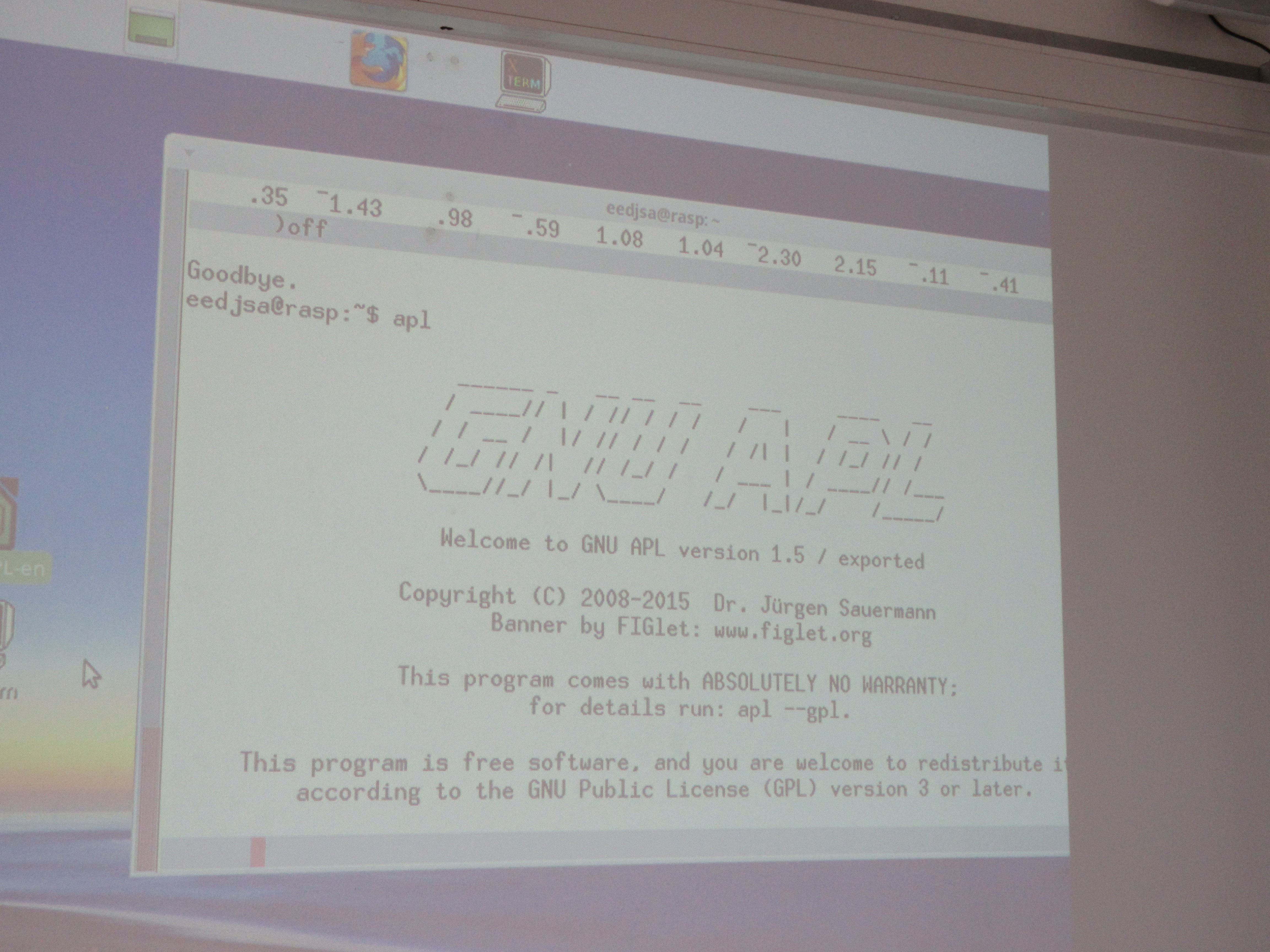
The results of this work are now available in the GitHub Repository Dyalog/Selenium. The following example, included in that repository, shows a simple test which verifies that the TryAPL website is able to execute a simple expression:
 ∇ r←Basic;S;result
 ⍝ Basic test that TryAPL is working - return error message if it isn't

 S←##.Selenium
 S.InitBrowser''
 S.GoTo'http://tryapl.org'

 'APLedit'S.SendKeys'1 2 3+4 5 6'
 S.('APLedit'SendKeys Keys.Return)
 result←'ClassName'S.Find'result'
 r←result S.WaitFor'5 7 9' '1 2 3+4 5 6 failed'
 ∇
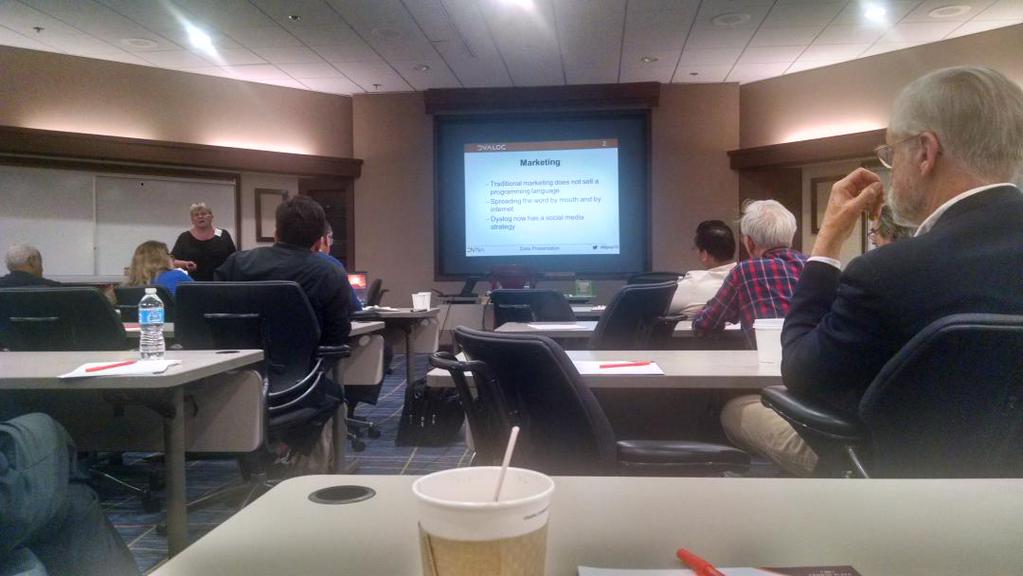
MiServer Regression Testing
The primary motivation for this work has been to create regression test scripts for MiServer version 3.0. The MiServer regression testing mechanism is extremely simple (possibly a bit TOO simple, we’ll cross that bridge later): If a site contains a folder called “QA”, and the folders within mirror the structure of the web site, then a mechanism exists to load each page in turn and run the corresponding test function. You can read more about it on GitHub and see it working in the video at the top of this post.
 Follow