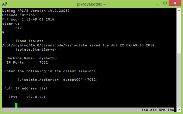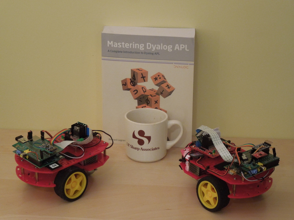

This blog originally started when I took delivery of the DyaBot, a Raspberry Pi and Arduino based variant of the C3Pi running Dyalog v13.2. The architecture of the ‘bot and instructions for building your own inexpensive robot can all be found in blog entries from April to July of last year.
The downside of only using inexpensive components is that some of them are not very precise. The worst problem we face is that the amount of wheel movement generated by the application of a particular power level varies from one motor to the next, and indeed from moment to moment. Trying to drive a specific distance in a straight line, or make an exact 90 degree turn regardless of the surface that the ‘bot is standing on, are impossible tasks with the original Dyabot. You can have a lot of fun, as I hope the early posts demonstrate, but we have higher ambitions!
Our next task is to add motion sensors to the DyaBot, with a goal of being able to measure actual motion with sufficient accuracy to maintain our heading while driving straight ahead – and to make exact turns to new headings, like the 90-degree turn made in this video (the ‘bot has been placed on a Persian carpet to provide a background containing right angles):
Introducing the MPU-6050
For some time we have had an MPU-6050, which has 3-axis rotation and acceleration sensors, attached to our I2C bus, but haven’t been able to use it. About ten days ago (sorry, I took a few days off last week), @RomillyC came to visit us in Bramley to help me read some Python code that was written for this device. The current acceleration or rotation on each axis is constantly available as a register and can be queried via I2C. Translated into APL, the code to read the current rate of rotation around the vertical axis is:
 ∇ r←z_gyro_reading ⍝ current z-axis rotation in degrees
   r←(read_word_2c 70)÷131 ⍝ Read register #70 and scale to deg/sec
 ∇

 ∇ r←read_word_2c n;zz
   r←I2 256⊥read_byte_2c¨n+0 1               ⍝ Read 2 registers and make signed I2
 ∇

 ∇ r←read_byte_2c n;z
   z←#.I2C.WriteArray i2c_address (1,n)0     ⍝ Write register address
   r←2 2⊃#.I2C.ReadArray i2c_address (1 0)1  ⍝ Read input
 ∇

 I2←{⍵>32767:1-65535-⍵ ⋄ ⍵} ⍝ 16-bit 2's complement to signed
Integrating to Track Attitude
Reading the register directly gives us the instantaneous rate of rotation. If we want to track the attitude, we need to integrate the rates over time. The next layer of functions allows us to reset the attitude and perform very primitive integration by multiplying the current rotation with the elapsed time since the last measurement:
∇ r←z_gyro_reset            ⍝ Reset Gyro Integration
  z_gyro_time←now           ⍝ current time in ms
  z_gyro_posn←0             ⍝ current rotation is 0
∇

∇ r←z_gyro;t;delta          ⍝ Integrated gyro rotation
  t←now                     ⍝ current time in ms
  delta←0.001×t-z_gyro_time ⍝ elapsed time in seconds
  r←z_gyro_posn←z_gyro_posn+delta×z_gyro_reading+z_gyro_offset
  z_gyro_time←t             ⍝ last time
∇
We can now write a function to rotate through a given number of degrees (assuming that the gyro has just been reset): we set the wheels in motion, monitor the integrated angle until we are nearly there, then shut off the engines. We continue logging the angles for a brief moment to monitor the deceleration. The function returns a two-column matrix containing the “log” of rotation angles and timestamps:
    ∇ log←rotate angle;bot;i;t

      log←0 2⍴0 ⍝ Angle, time
      bot.Speed←3 ¯3 ⍝ Slow counter-clockwise rotation

      :Trap 1000 ⍝ Catch interrupts
          :Repeat
              log⍪←(t←z_gyro),now
          :Until t>angle-7 ⍝ Stop rotating 7 degrees before we are done
      :EndTrap

      bot.Speed←0 ⍝ cut power to the motors
      :For i :In ⍳25 ⍝ Capture data as we slow down
          log⍪←z_gyro,now
      :EndFor
    ∇
The logged data from the rotation captured in the video at the top is charted below:
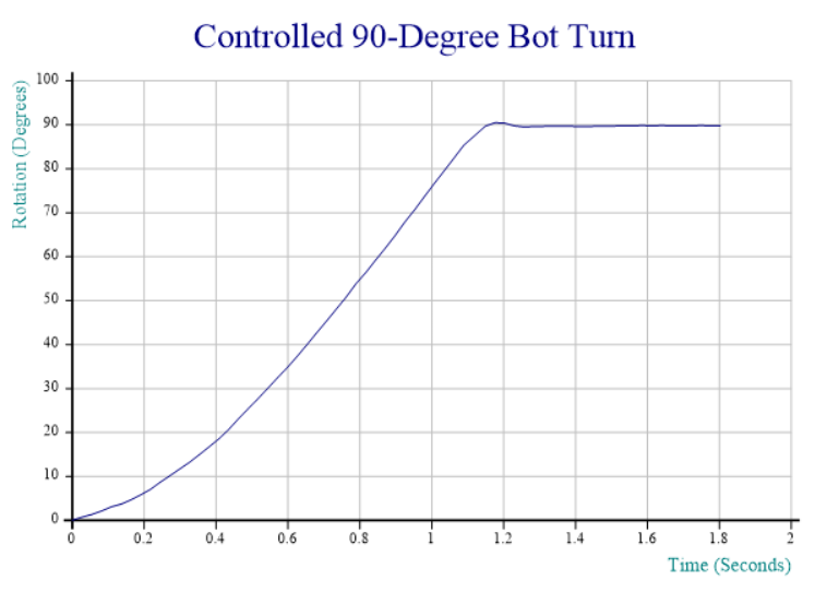 Even with the primitive integration and rotation strategies, the results already look quite promising. I’ll be taking most of this week off – part of it without access to the internet(!), but once I am back, expect the next blog entry to explore writing functions that accelerate and slow down in a more controlled fashion as well as stop at the right spot rather than relying on a specific amount of friction to rotate through the last 7 degrees (note the very slight reverse rotation at the end, probably caused by the Persian carpet being a bit “springy”). I will also clean up the code and post the complete solution on GitHub – and perhaps even look at some better integration techniques.
If you would like to make sure you don’t miss the next installment, follow the RSS feed or Dyalog on Twitter.
 Follow