Creating Shortcuts (Microsoft Windows)

At Dyalog, a developer not only needs access to all of the readily available editions of the interpreter but also to earlier versions that are no longer officially supported. On my Microsoft Windows Desktop I have a folder that contains a shortcut to my developer builds of all these interpreters.

I’ve recently suffered a complete failure of my C drive which, of course, contained my Windows desktop and all my shortcuts – which were lost.

The Dyalog interpreter exists in Classic and Unicode editions and 32 and 64 bit flavours…for versions from 12.0 to 14.1 this is a total of 28 interpreters. I couldn’t bring myself to create each of those 28 shortcuts by hand; let’s not even consider that if I were to build both debug and optimised binaries that would be 56 shortcuts!

Fortunately we have an old COM example (in the shortcut.dws workspace) which is shipped with the product. It’s a trivial exercise to call the supplied SHORTCUT function in one or more (ahem!) loops to create all the required shortcuts:

 Dyalogs;vers;chars;bits;location;v;c;b;dyalog;dir;name

 vers←'12.0.dss' '12.1.dss' '13.0.dss' '13.1.dss' '13.2.dss' '14.0.dss' 'trunk'
 chars←'classic' 'unicode'
 bits←'32' '64'

 ⎕NA'u shell32|SHGetFolderPath* u u u u >0T'
 location←'\Dyalog',⍨2⊃SHGetFolderPath 0 0 0 0 255

 :For v :In vers
     :For c :In chars
         :For b :In bits

             dir←'e:\obj\',v,'\2005\apl\win\',b,'\',c,'\winapi\dev\dbg'
             dyalog←dir,'\dyalog.exe'
             name←'.lnk',⍨location,'\',({v↓⍨('.dss'≡¯4↑v)/¯4}v),' ',b,' ',c

             name SHORTCUT dyalog dir'' 1('' 0)0 ''
         :End
     :End
 :End

shortcuts

Aligning Diff Output

‘Bots are off limits this week so here is a story from this year’s Iverson College – a fantastic week spent in the company of a wonderful mixture of array and functional language gurus and newbies, all learning from each other. One evening, Dhru Patel presented a problem that he was working on which involved displaying the results of a “diff” side by side with the matched rows aligned. For example, the input might be:

      OLD NEW
┌────────┬────────┐
│This    │This    │
│is the  │original│
│original│is not  │
│text    │        │
└────────┴────────┘

Edited by Yoda, the text was. The selection of rows to be aligned requires finding the longest sequence of rows from the original data that matches rows in the edited data without ever skipping backwards through either sets of data. In this case, it is the original first and third row, matching the first two edited rows. We will return to how we might identify these rows in a future blog entry (meanwhile, try to grok John Scholes’ YouTube video on Depth First Searching and think about it). For now, we will provide this information as a left argument, a vector of Boolean vectors that marks the location of the matched rows:

      (1 0 1 0)(1 1 0) AlignMatched OLD NEW
┌────────┬────────┐
│This    │This    │
│is the  │        │
│original│original│
│text    │        │
│        │is not  │
└────────┴────────┘

At Iverson College there was general agreement that “there should be a non-looping solution”, and Devon McCormick immediately stated that he would bet that it involved grade (). Let us explore:

      masks←(1 0 1 0)(1 1 0)
      ⎕←matched←∊masks ⍝ The two match masks catenated together
 1 0 1 0 1 1 0 
      ⎕←origin←(≢¨OLD NEW)/0 1 ⍝ 0 for items from the old array, 1 for new
 0 0 0 0 1 1 1 
      ⎕←block←∊+\¨masks ⍝ running count of matched rows
 1 1 2 2 1 2 2   
      ⎕←data←block,(~matched),origin,OLD⍪NEW
1 0 0 This    
1 1 0 is the  
2 0 0 original
2 1 0 text    
1 0 1 This    
2 0 1 original
2 1 1 is not  

Our goal is to create an expansion mask for each argument; this is going to insert blank lines at the points where a non-matched row from the other argument is included. The next step is to reorder everything by ascending block number, and within each block move the matched rows to the front (ascending by ~matched), as follows:

      ⎕←data←data[⍋data[;1 2];]
1 0 0 This    
1 0 1 This    
1 1 0 is the  
2 0 0 original
2 0 1 original
2 1 0 text    
2 1 1 is not 

This contains all the items from both texts in the order that they would need to appear in the final results. We can extract the reordered flag vectors:

       matched←~data[;2] ⋄ origin←data[;3]

Now, (origin=0) is an expansion mask that would expand OLD to match the above, and (origin=1) would do the same for NEW:

      0 1 {(origin=⍺)⍀⍵}¨OLD NEW
┌────────┬────────┐
│This    │        │
│        │This    │
│is the  │        │
│original│        │
│        │original│
│text    │        │
│        │is not  │
└────────┴────────┘

To align the matched rows, we need to eliminate inserted blanks that correspond to matched rows from the other side:

      0 1{((~matched∧origin≠⍺)/origin=⍺)⍀⍵}¨OLD NEW
┌────────┬────────┐
│This    │This    │
│is the  │        │
│original│original│
│text    │        │
│        │is not  │
└────────┴────────┘

In the final function, which collects the relevant lines of code from our experiments, we do not create the temporary “data” matrix, but reorder the origin and matched vectors individually – and instead of doing grade up on a two-column matrix, we compute an integer vector that will sort by descending matched within ascending block (because we know that grade up on a simple small-range integer vector will run like greased lightning):

 AlignMatched←{                ⍝ align matched rows of 1⊃⍵ and 2⊃⍵
     matched←∊⍺                ⍝ matches are marked by 1⊃⍺ and 2⊃⍺
     origin←(≢¨⍵)/0 1          ⍝ identify origin of items in matched (0=old. 1=new)
     block←∊+\¨⍺               ⍝ running count of matched rows
     order←⍋(2×block)-matched  ⍝ Order so matching rows are adjacent and order of
     (origin matched)←(⊂⊂order)⌷¨origin matched ⍝ items following matched row is preserved
     0 1{((~matched∧origin≠⍺)/origin=⍺)⍀⍵}¨⍵ ⍝ Expand exluding matched from "other" list
 }


Reviving Lost Arts

The algorithm above makes use of techniques that were well-known in APL circles in the 1980s, but atrophied after nested arrays arrived on the scene and applications tended to keep parts of the data in separate leaves of an array rather than using simple data structures.

If you would like to read up on some of the old techniques, you might enjoy browsing the FinnAPL Idiom Library, and Bob Smith’s immortal Boolean Functions and Techniques. Although nested arrays might have made them a little less relevant in the 90s and 00s, the search for high-performance parallel solutions could bring them back, as explained in this session from Dyalog ’12, on Segmented Scans and Nested Data Parallelism by Andrzej Filinski.

APL-Controlled Robot Performs Death-Defying Stunts Using PiCam

Regular readers will remember my whining about the poor precision of both infra-red and ultrasonic sensors. But today, the Raspberry Pi / Dyalog APL – controlled “DyaBot” was observed driving on a dinner table – where the slightest navigational error could mean a 3-foot plunge and certain death! How can this be?

The answer is: the “PiCam” finally arrived last week!!!

Capturing Images with The PiCam

I no longer need to complain about sonar beams being up to 30 degrees wide: the PiCam has a resolution of up to 1080×1920 pixels! So all we need is some software to interpret the bits…First, we capture images using the “raspistill” command:

raspistill -rot 90 -h 60 -w 80 -t 0 -e bmp -o ahead.bmp

The parameters rotate the image 90 degrees (the camera is mounted “sideways”), set the size to 60 x 80 pixels (don’t need more for navigation), take the picture immediately, and store the output in a file called “ahead.bmp”. (Documentation for the camera and related commands can be found on the Raspberry Pi web page.) Despite the small number of pixels, the command takes a full second to execute – anyone who knows a way to speed up the process of taking a picture, please let me know!

In the video, each move takes about 3 seconds, this is simply because each cycle is triggered by a browser refresh of the page after 3 seconds. Capturing the image takes about 1 second, the “image analysis” about 40 milliseconds, so we could be driving a lot faster with a bit of Javascript on the client side (watch this space).

Extracting BitMap Data

Under Windows, Dyalog APL has a built-in object for reading BitMap files, but at the moment, the Linux version does not have an equivalent. Fortunately, extracting the data using APL is not very hard (after you finish reading about BMP files on WikiPedia):

tn←'ahead.bmp' ⎕NTIE 0     ⍝ Open "native" file
(offset hdrsize width height)←⎕NREAD tn 323 4 10 
                           ⍝ ↑↑↑ Read 4 Int32s from offset 10
data←⎕NREAD tn 80 (width×height×3) offset ⍝ Read chars (type 80)
data←⊖⎕UCS(height width 3)⍴data ⍝ Numeric matrix, reverse rows

The above gives us a 60 by 80 by 3 matrix containing (R,G,B) triplets. This code assumes that BMP file is in the 24-bit format created by raspistill; I will extend the code to handle all BMP formats (2, 16 and 256 colours) and post it when complete – but the above will do for now.

Where’s the Edge?

At Iverson College last week, I demonstrated the DyaBot driving on a table with a green tablecloth, using code which compared the ratio between R,G,B values to an average of a sample of green pixels from one shot. Alas, I prepared the demo in the morning and, when the audience arrived, there was much more (yellowish) light coming in through the window. This changed the apparent colour so much that the bot decided that the side of the table facing the window was now unsafe, and it cowered in the darkness.

Fortunately, I was talking to a room full of very serious hackers, who sent me off to Wikipedia to learn about “kernels” as a tool for image processing. Armed with a suitable edge detection kernel, I was able to test this new algorithm on a dozen shots taken at different angles with the PiCam. Each pair of images below has the original on the left, and edges coloured red on the right. Notice that, although the colour of the table varies a lot when viewed from different directions – especially when there is background glare – the edges are always correctly identified:

Edge Detection Examples

Except for the image at the bottom left, where the bot is so close to the edge that the table is not visible at all (and the edge is the opposite wall of the room, ten feet away), we seem to have a reliable tool.

The PiServer Page

The code to drive the bot is embedded in a “PiServer” (MiServer running on a Rasperry Pi) web page. Each refresh of the page takes a new picture, extracts the bits, and calls the main decision-making function. The suggested action (turn or drive straight ahead) is displayed in the form, and the user has the choice of pressing OK to execute the command, pressing the “Nah” button to take a new photo and try again (after moving the bot, changing the lighting in the room, or editing the code). There are also four “manual” buttons for moving the Bot. After testing the decision-making abilities of the code, brave programmers press the “Auto” button, allowing the robot to drive itself without waiting for confirmation before each command (see the video at the start of this post)!

Robot Views Table at Dyalog House

The Code

The central decision-making function and the kernel computation function are listed below. The full code will be uploaded to the MiServer repository on GitHub, once it is finally adjusted after I find a way to attach the PiCam properly, rather than sticking it to the front of the Bot with a band-aid!

∇ r←StayOnTable rgb;rows;cols;table;sectors;good;size;edges
 ⍝ Based on input from PiCam, drive at random, staying on table
 ⍝ Return vector containing degrees to turn and 
 ⍝               #seconds to drive before next analysis

 (rows cols)←size←2↑⍴rgb
 ⍝ First detect edges in each colour separately
 edges←EdgeDetectAll∘AK¨⊂[1 2]rgb
 ⍝ Call it an edge if any r, g or b result is >75% of original
 edges←∨/(↑[0.5]edges)>0.75×1 1↓¯1 ¯1↓rgb
 ⍝ Look for lowest edge in each column 
 table←+⌿∧⍀~⊖edges
 ⍝ Divide into 3 equally sized sectors (left, centre, right) 
 sectors←((⍴table)⍴(⌈(⍴table)÷3)↑1)⊂table
 ⍝ Find the LOWEST edge in each sector
 good←⌊/¨sectors

 :If good∧.>15 ⍝ More than 15 pixel rows of table in all sectors
    r←0,0.1⌈(good[2]-15)÷25 ⍝ Carry straight on for a while
 :Else ⍝ Some sectors have less than 15 pixel rows
    :If 0≠1↑previous ⋄ r←previous 
        ⍝ Once started turning, keep turning the same way
    :Else 
        r←((1+>/good[1 3])⊃45 ¯45),0 ⍝ Turn in "best" direction
    :EndIf
 :EndIf
 previous←r ⍝ Remember last turn for next decision
∇

The function AK (Apply Kernel), and the kernel are defined as follows:

∇ r←kernel AK data;shape
   shape←⍴kernel
   r←(1-shape)↓⊃+/,kernel×(¯1+⍳1↑shape)∘.⊖(¯1+⍳1↓shape)∘.⌽⊂data
∇

 EdgeDetectAll ⍝ Our 3x3 kernel
¯1 ¯1 ¯1
¯1  8 ¯1
¯1 ¯1 ¯1

Note the similarity of AK to the APL Code for Conway’s Game of Life!


PiServer at Thor8.dk

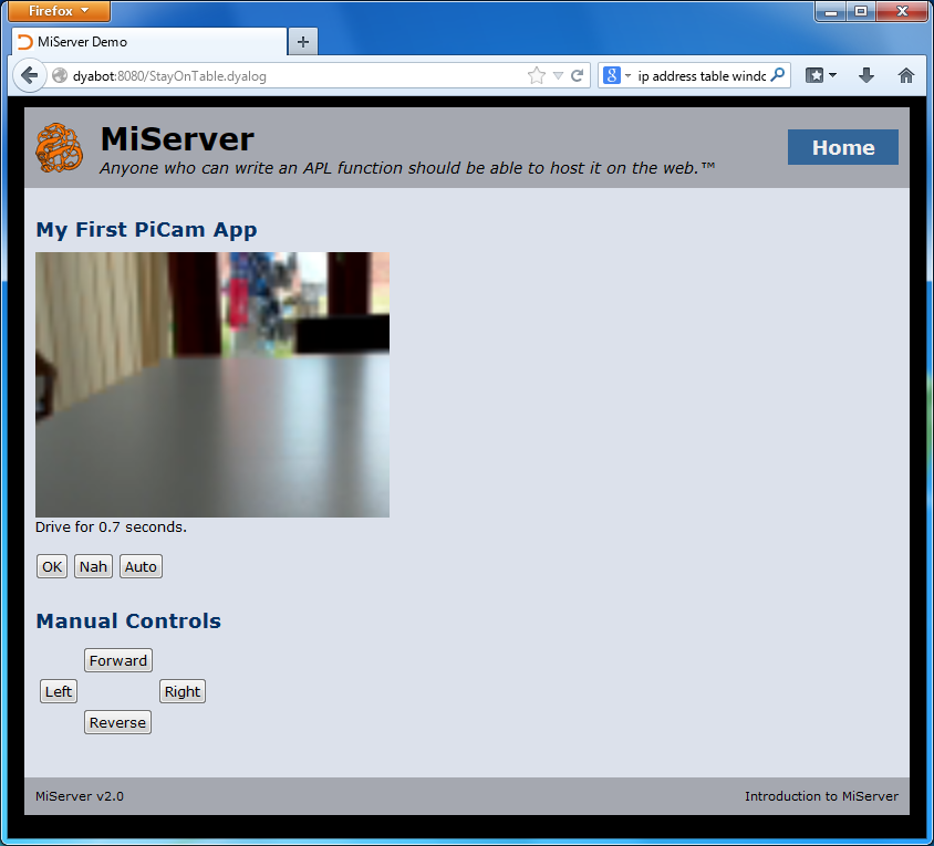
I’ve been wanting to run a Web Server from my home for many years. In fact, I have been paying for the domain Thor8.dk (my street address is Thorsvænget 8), and a fixed IP address for 5 years now – without getting it implemented. But today, with a little help from Jason Rivers who helped me set it up so it starts automatically on reboot, I have been able to deploy a MiServer – a web framework written entirely in Dyalog APL – on my Raspberry Pi (the one that is not embedded in the DyaBot) – at the address http://thor8.dk. Please be gentle with it, it is a very small machine on a regular ISP connection with only 1Mb upload capacity!

MiServer + Raspberry Pi = PiServer

The MiServer is a project that has been evolving for the last several years, with the goal of putting web application development in easy reach of those APL developers who are not also comfortable with mainstream web technologies like Microsoft IIS / ASP.NET, Apache, PHP etc. It is a web framework written entirely by APLers, for APLers – as an open-source project which is now available at https://github.com/Dyalog/MiServer. The motto of this project is that “Anyone who is able to write an APL function should be able to host it on the web”.

The site at “thor8” is a slightly modified version of the demo site that is included with the MiServer installation. Note that one of the features of the site is that, from any page, if you click on the Viking amulet in the top left corner, you can see the source code for the page. If you’d like to learn more about the MiServer, the User Guide is also available on GitHub.

The Mortgage Example

A contributing factor to my finally getting my act together this week is that Nick Nickolov’s NGN/APL project, is an APL interpreter written in CoffeeScript, sparked a thread that has been running on LinkedIn for a while, which included a discussion on alternative mechanisms for implementing web apps in APL. While I think Nick’s project is very cool, and I look forward to meeting him at Iverson College next week, I could not avoid feeling a powerful urge to demonstrate that it now straightforward to write interactive web sites using a state-of-the art, industrial strength APL system. Many thanks to Brian Becker, who has done most of the work on recent features of the MiServer (and is currently working on MiServer 3.0 which aims to make the development of web pages much more similar to desktop application development), for his assistance in putting together the example.If the PiServer is still up and running you can view the example at http://thor8.dk/mortgage. Here is an image, just in case it isn’t:

PiServer Mortgage

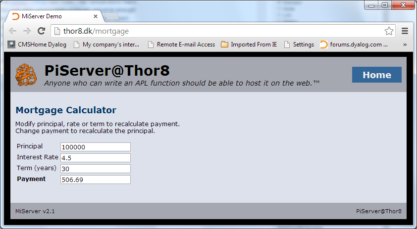
If you modify the principal amount, interest rate or the term, the calculator will calculate a new monthly payment. If you adjust the payment to something that you can afford, the principal amount will be adjusted accordingly.

The Code

As previously mentioned, if you click on the orange amulet at the top left, the code for the page will be displayed. I’d like to explain selected lines of the code here:

:Class mortgage : MiPage

Every MiServer Page (MiPage) is a Dyalog APL class which derives from the base class MiPage. This base class adds the CSS (style sheet) and behaviour like the display of code.

Public Fields

    :Field Public event         ⍝ the triggered event
    :Field Public what          ⍝ the id of the element
    :Field Public prin←'100000' ⍝ principal field
    :Field Public rate←'4.5'    ⍝ rate
    :Field Public term←'30'     ⍝ term (years)
    :Field Public pmt←''        ⍝ payment

The main job of the MiServer is to move values arriivng from the browser, in the form of fields in an HTML form, or JSON data, to instance variables in your class. You need to name the fields that you want the MiServer to look for in order for this to happen (you can also retrieve other values using API function calls, but that is a longer story).

Application Code

tonum←{{(,1)≡1⊃⍵:2⊃⍵ ⋄ ''}⎕VFI ⍵} ⍝ check for a single number
calcpmt←{0::'Err' ⋄ p r n←⍵÷11200(÷12) ⋄ .01×⌈100×p×r÷1-(1+r)*-n}
calcprin←{0::'Err' ⋄ r n m←⍵÷1200(÷12)1 ⋄ .01×⌈100×m÷r÷1-(1+r)*-n}

These three lines of code are the actual application code – one function to compute the payment based on principal, rate and term – and another to calculate the principal based on the other three values.

Defining The Form

 inputs←1 2⍴'Principal'('prin'Edit prin) 
 inputs⍪←'Interest Rate'('rate'Edit rate)
 inputs⍪←'Term (years)'('term'Edit term)
 inputs⍪←'<b>Payment</b>'('pmt'Edit pmt)
 html,←'id="mortgage"'('POST'Form)Table inputs

Within the function Render, which is called when the page is rendered, these lines of code create a 4×2 nested array containing labels in the first column, and HTML edit fields in the 2nd column. The function Table wraps an HTML table around this array and the Form operator wraps that inside a form which will use the POST method (although in this case, that actually never happens, we drive all activities of change events on the edit fields).

Wiring up the Callbacks

  selector←'#mortgage input'
  event←'change'
  returndata←'formdata' '#mortgage' 'serialize'
  html,←req #.JQ.On selector event returndata

These four lines of code set up a client-side JavaScript callback using a technology called JQuery, which will post a serialised copy of the form back to the server using an “AJAX” style transaction (we call it “APLJAX”). In a larger form we might want to be more selective about what we send back, but in this case the entire serialised form is still a very small amount of data.

Updating the Form

    :CaseList 'prin' 'rate' 'term' 
       resp←('execute'('$("#pmt").val("',(⍕calcpmt p r n),'")'))
    :Case 'pmt' ⍝ payment changed, calculate principal
       resp←('execute'('$("#prin").val("',(⍕calcprin r n m),'")'))

The above lines are “the beef” in terms of the interaction: A response is constructed which will cause the value of either the pmt or the prin field to be updated, by sending a snippet of JavaScript back to the client to be executed dynamically.

We are actually working hard to eliminate the use of the above feature (the ability to execute JavaScript), because we don’t think most APLers will want to learn even this amount of JS. If you can make do with two buttons marked “Calculate payment” and “Adjust Principle”, rather than reacting each time a field is changed, no JS is required – as is the case for most of the other MiServer sample pages. Version 3.0 of MiServer will hopefully have a mechanism to update values of selected parts of the DOM without injecting JS. However, this example should hopefully demonstrate that you can write an APL server-side application which does *anything* using this technology.

Please take it for a spin – we are happy to receive comments on this blog, or via e-mail to apltools at dyalog dot com.

The DyaBot will of course be running a PiServer too. More about that next week, the bot is also coming to Iverson College.


APL at work in Africa

My dad is originally from the Cape, and I grew up in Botswana, so hopefully I can be forgiven for feeling that it is very cool to find Dyalog APL at the core of a project which aims to increase financial literacy and support the financial stability of small and medium-sized enterprises in South Africa, by delivering a “cash flow optimizer” on phones and tablets:

More Links:

CF04i Home Page
Article in the Financial Mail Corporate Essentials
Riskflow Blog

Elementary Cellular Light-Emitting Automaton

In response to an earlier post on driving an 8-bar LED using the Raspberry Pi, Roger Hui commented that 8 lights should be sufficient to display the output of a 1-d Game of Life. The code snippets displayed in this post are based on some working code that Roger was also kind enough to forward to me.

The following two functions provide the basic building blocks for the computation of the next generation of a 1-d cellular automaton:

bits←{(8⍴2)⊤⍵}           ⍝ Encode a number as 8 binary bits
neighbors←{↑¯1 0 1∘.⌽⊂⍵} ⍝ Map vector => 3-row matrix with neighbors

These allow us to perform the following transformations:

      bits 5
0 0 0 0 0 1 0 1
      bits 110
0 1 1 0 1 1 1 0
      neighbors b←0 1 0 0 1 1 1 1
1 0 1 0 0 1 1 1
0 1 0 0 1 1 1 1
1 0 0 1 1 1 1 0
      2⊥neighbors b ⍝ base-2 decode of each column
5 2 4 1 3 7 7 6

With these, it is now easy to define a function to compute the next generation of a pattern for a given Wolfram Code (and test it with a couple of arguments):

      wc←{(bits ⍺)[8-2⊥neighbors ⍵]}
      110 wc b
1 1 0 1 1 0 0 1
      110 wc 110 wc b ⍝ 3rd generation
0 1 1 1 1 0 1 1

We subtract the result of the base-2 decode from 8, because the least significant bit (bit 0) is the 8th element of the vector returned by the bits function. Next, we define an operator which returns a matrix containing a number of generations:

    ∇ r←gens(rule wcgm)pattern;i
[1] ⍝ Wolfram Code Generations
[2]
[3] r←(gens,⍴pattern)⍴pattern
[4] :For i :In 1↓⍳gens
[5]    r[i;]←rule wc r[i-1;]
[6] :EndFor
    ∇

    5 (110 wcg) b ⍝ 5 generations of code 110
0 1 0 0 1 1 1 1
1 1 0 1 1 0 0 1
0 1 1 1 1 0 1 1
1 1 0 0 1 1 1 1
0 1 0 1 1 0 0 0

Finally, we can add 1 to the boolean matrix and use it to index into a 2-element character vector, to get better “visualization” of the result (10 generations of Wolfram code 20):

      '-*'[1+10 (20 wcgm) b]
-*--****
-**-----
---*----
---**---
-----*--
-----**-
-------*
*------*
-*------
-**-----

The function also works with longer inputs – in the example below a random input of length 60 (20 generations of Wolfram code 18, this time using just blank and asterisk for the display):

     ' *'[1+20 (18 wcgm) 1=?60⍴2]
*****    * ***** *** ** *  * ***    *  *** *  ***  ** ***** 
     *  *                **     *  * **     **   **         
    * ** *              *  *   * **    *   *  * *  *        
   *      *            * ** * *    *  * * * **   ** *       
  * *    * *          *        *  * **        * *    *      
 *   *  *   *        * *      * **    *      *   *  * *     
* * * ** * * *      *   *    *    *  * *    * * * **   *    
              *    * * * *  * *  * **   *  *        * * *  *
*            * *  *       **   **    * * ** *      *     ** 
 *          *   ** *     *  * *  *  *        *    * *   *   
* *        * * *    *   * **   ** ** *      * *  *   * * *  
   *      *     *  * * *    * *       *    *   ** * *     **
* * *    * *   * **     *  *   *     * *  * * *      *   *  
     *  *   * *    *   * ** * * *   *   **     *    * * * **
*   * ** * *   *  * * *          * * * *  *   * *  *        
 * *        * * **     *        *       ** * *   ** *      *
    *      *      *   * *      * *     *      * *    *    * 
   * *    * *    * * *   *    *   *   * *    *   *  * *  * *
* *   *  *   *  *     * * *  * * * * *   *  * * * **   **   
   * * ** * * ** *   *     **         * * **        * *  * *


Finally, we can light the lights using the BarLED class from our GitHUB repository – and the Quick2Wire interface board and LED Bar – see the original post for an explanation. The video below shows the output resulting from the following APL expressions

      ]load /home/pi/BarLED
      bl←⎕NEW BarLED ⍬
      0.2 bl.Play ↓50(20 wcg) 0 1 0 0 1 1 1 1
      0.2 bl.Play ↓50(18 wcg) 0 1 0 0 1 1 1 1

Many thanks to Roger for the inspiration to take this one step further (and the code)! For a 2-dimensional implementation of Conway’s classic Game of Life, see the video by John Scholes at http://www.youtube.com/watch?v=a9xAKttWgP4.