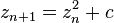
It amazes me that an equation so simple can produce images so beautiful and complex.  I was first introduced to the Mandelbrot set by the August 1985 issue of Scientific American. Wikipedia says “The Mandelbrot set is the set of complex numbers ‘c’ for which the sequence ( c , c² + c , (c²+c)² + c , ((c²+c)²+c)² + c , (((c²+c)²+c)²+c)² + c , …) does not approach infinity.” This means that in the images below, the areas in black are points in the Mandelbrot set and the other point colors are determined by how quickly that point “zooms” off towards infinity. The links above give a deeper discussion on the Mandelbrot set – for this post I’d like to focus on how I was able to speed my Mandelbrot set explorer up using isolates.

I find I learn things more easily through application than abstraction. In 2006 I wanted to learn more about the built-in GUI features of Dyalog for Windows and the application I chose was a Mandelbrot set explorer. While the basic algorithm for calculating a point in the Mandelbrot set is fairly simple, a 640×480 pixel image could involve over 75 million calculations. As new versions of Dyalog are released, I try to experiment with any applicable new features and possibly incorporate them into the explorer. For instance, when complex numbers were introduced in Dyalog, I modified the explorer to use them.

Dyalog v14.0 introduced a prototype of a parallel computing feature called isolates that may one day be integrated into the interpreter. Isolates behave much like namespaces except that they run in their own process with their own copy of the interpreter. Each process can run on a separate processor, greatly improving performance. You can even set up isolate servers on other machines.

Mandelbrot set calculations are ideal candidates for parallelization as:

• they’re CPU intensive
• each pixel can be calculated independently of others
• there are no side effects and no state to maintain

The core calculation is shown below. It takes the real and imaginary parameters for the top left corner, the height and width of the image and the increment along each dimension and uses those parameters to build a set of co-ordinates, then iterates to see how quickly each co-ordinate “escapes” the Mandelbrot set.

 ∇ r←real buildset_core imaginary;height;i_incr;top;width;r_incr;left;set;coord;inds;cnt;escaped
  ⍝ Calculate new Mandelbrot set - remember using origin 0 (⎕IO←0)
  ⍝ real and imaginary are the parameters of the space to calculate
  ⍝       real            imaginary
  ⍝ [0]   width           height            of the image
  ⍝ [1]   increment size  increment size    along each axis
  ⍝ [2]   top             left              coordinates

   (height i_incr top)←imaginary            ⍝ split imaginary argument parameters
   (width r_incr left)←real                 ⍝ split real argument parameters
   set←coord←,(0J1×top+i_incr×⍳height)∘.+(left+r_incr×⍳width) ⍝ create all points in the image
   inds←⍳≢r←(≢coord)⍴0                      ⍝ initialize the result and create vector of indices
   :For cnt :In 1↓⍳256                      ⍝ loop up to 255 times (the size of our color palette)
       escaped←4<coord×+coord               ⍝ mark those that have escaped the Mandelbrot set
       r[escaped/inds]←cnt                  ⍝ set their index in the color palette
       (inds coord)←(~escaped)∘/¨inds coord ⍝ keep those that have not yet escaped
       :If 0∊⍴inds ⋄ :Leave ⋄ :EndIf        ⍝ anything left to do?
       coord←set[inds]+×⍨coord              ⍝ the core Mandelbrot computation... z←(z*2)+c
   :EndFor
   r←(height,width)⍴r                       ⍝ reshape to image size
 ∇

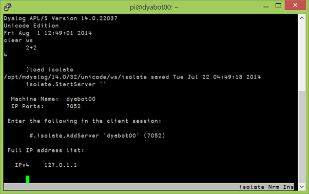
So, what’s involved in using isolates to parallelize the explorer?  As it turns out, not much! First I )COPYed the isolate namespace from the isolate workspace distributed with Dyalog v14.0. I wanted to be able to select the number of processors to use, so I added a line to my init function to query how many processors are available:

 processors←1111⌶⍬ ⍝ query number of processors

Next I wrote a small function to initialize isolates for as many processors as were selected (2 or more). Notice that when creating the isolates, I copy buildset_core (from above) into each one:

 ∇ init_isolates processors
  ⍝ called upon initialization, or whenever user changes number of processors to use
   f.isomsg.Visible←1    ⍝ turn form's "Isolates initializing" message on
   {}isolate.Reset''     ⍝ reset the isolates
   {}isolate.Config'processors'processors ⍝ set the number of processors
   :If processors>1      ⍝ if using more than one processor
       ⍝ create the isolates, populating each one with buildset_core
       isolates←isolate.New¨processors⍴⎕NS'buildset_core'
   :EndIf
   f.isomsg.Visible←0    ⍝ turn the form message off
 ∇

Finally, I wrote a routine to share the work between the selected number of processors and assemble the results back together.

 ∇ r←size buildset rect;top;bottom;left;right;width;height;vert;horz;rows;incr;imaginary;real
  ⍝ Build new Mandelbrot Set using isolates if specified
  ⍝ rect is the top, bottom, left, and right
  ⍝ size is the height and width of the image
   (top bottom left right)←rect
   (height width)←size
   vert←bottom-top                             ⍝ vertical dimension
   horz←right-left                             ⍝ horizontal dimension
   rows←processors{¯2-/⌈⍵,⍨(⍳⍺)×⍵÷⍺}height     ⍝ divide image among processors (height=+/rows)
   incr←vert÷height                            ⍝ vertical increment
   imaginary←↓rows,incr,⍪top+incrׯ1↓0,+\rows  ⍝ imaginary arguments to buildset_core
   real←width,(horz÷width),left                ⍝ real arguments to buildset_core
   :If processors=1                            ⍝ if not using isolates
       r←real buildset_core⊃imaginary          ⍝ build the image here
   :Else
       r←⊃⍪/(⊂real)isolates.buildset_core imaginary ⍝ otherwise let the isolates to it
   :EndIf
 ∇

The images below depicts what happens with 4 processors. Each processor builds a slice of the image and the main task assembles them together.

So, how much faster is it?  Did my 8 processor Intel Core i7 speed things up by a factor of 8? No, but depending on where in the Mandelbrot set you explore, the speed is generally increased by at least a factor of 2 and sometimes as high as 5 or 6. I thought about why this might be and have a couple of ideas…

• There’s overhead to receive and assemble the results from each isolate.
• The overall time will be the maximum of the individual times; if one slice is in an area that requires more iterations, then the main task needs to wait for those results, even if the other slices have already finished. I could possibly show this by updating the individual slices as they become available. Maybe next time 🙂

What impressed me was that I could speed up my application significantly with about 20 lines of code and maybe an hour’s effort – most of which was spent tinkering to learn isolates. You can download the Mandelbrot set explorer from my GitHub repository.

Follow