
It is still true that most APL users live north of the equator, which means that at this time of year the sun is below the horizon more than half the time. It’s the perfect time to snuggle up in a warm place and watch some videos, and we’ll be offering you about three a week from now until just after the Winter Solstice, when we can start looking forward to the Spring.
As usual, we’ll be releasing videos of the vast majority of the presentations that were made at the recent Dyalog ’19 user meeting, which was held in Elsinore, Denmark in September. If you would like to get a feeling for what is coming, take a look at the blogs from the meeting itself, starting with this one.
In accordance with tradition, we’re opening with the three keynote presentations by Dyalog’s CEO Gitte Christensen, CTO Morten Kromberg, and Chief Architect John Daintree.
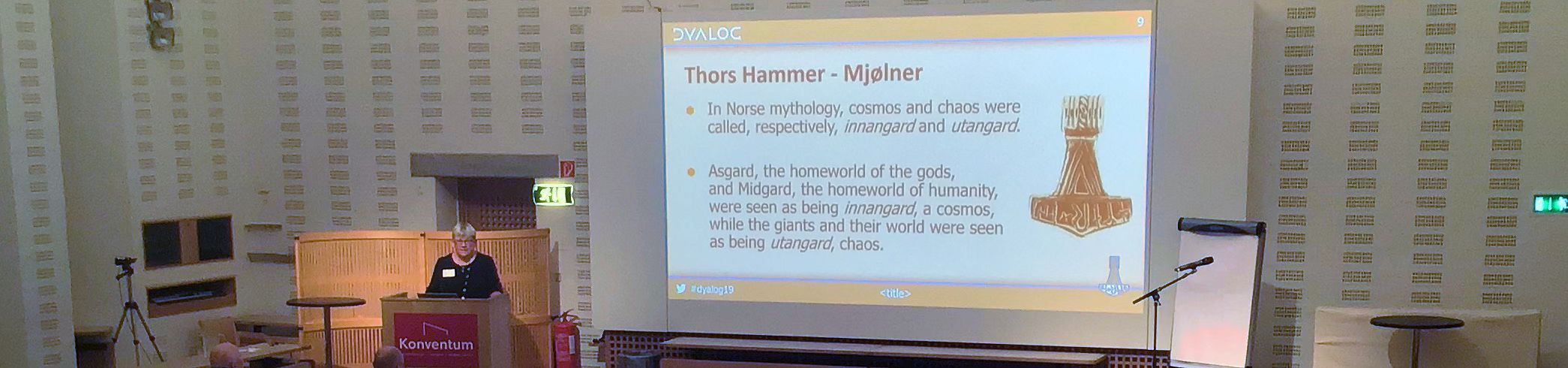
 2019 is the first “Year of the Hammer”: after seven years of Norse wyrms and seven years of Viking ships, we were now entering the era of seven hammer-inspired logos. As Gitte explains in her talk, we are celebrating the first year under Thor’s Hammer by making Dyalog APL freely available for non-commercial use – without requiring registration – under Microsoft Windows, Apple macOS and GNU/Linux (including a collection of public Docker images). The intention is to make APL much more easily accessible for experiments – especially in the cloud!
Gitte’s talk also contains sombre tones, remembering that we lost John Scholes in February as well as Harriett Neville, who had registered to attend Dyalog ’19 but passed away most unexpectedly just before the meeting.
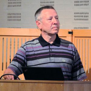 After last year’s Technical Road Map, which was almost entirely a live demonstration of using APL with modern development tools like Git, VS Code and Docker, I decided to play it safe this year and do no demos at all in my keynote. Instead, I concentrated on explaining some of our thoughts about making Dyalog APL easier to discover, learn and integrate into modern frameworks and development processes – and making applications written in APL easier to deploy and maintain. As a result, despite the world premiere of our new Webinar Jingle, composed by Stefano Lanzavecchia (short and long versions are available), I probably shocked the audience by leaving three minutes at the end for questions!
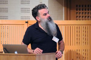 The title of John’s talk was “Cor(e) Blimey!”. The Cor(e) is of course a reference to Microsoft’s “.NET Core” but if English is not your first language, the title of John’s talk may need a little explanation. “Cor blimey” is an exclamation of surprise, a euphemism derived from “God Blind Me”. In this talk, John explains how Dyalog is poised to provide a bridge to Microsoft’s new portable, open source version of .NET. Scheduled for release with Dyalog version 18.0 next year, this will provide APL users with access to a vast collection of libraries under Linux and macOS, in addition to Windows.
Summary of this week’s videos:
- D01: Welcome to Dyalog ’19 (Gitte Christensen)
- D02: The Road Ahead (Morten Kromberg)
- D03: Cor(e) Blimey! What’s He Up To Now? (John Daintree)
I hope you enjoy these presentations. Join us again next week for another three recordings from Dyalog ’19!
 Follow