
Concluding Morten and Gitte’s whistlestop tour round Europe before heading to the US (see parts 1 and 2)
Saturday afternoon – Déjà Vu all over again…
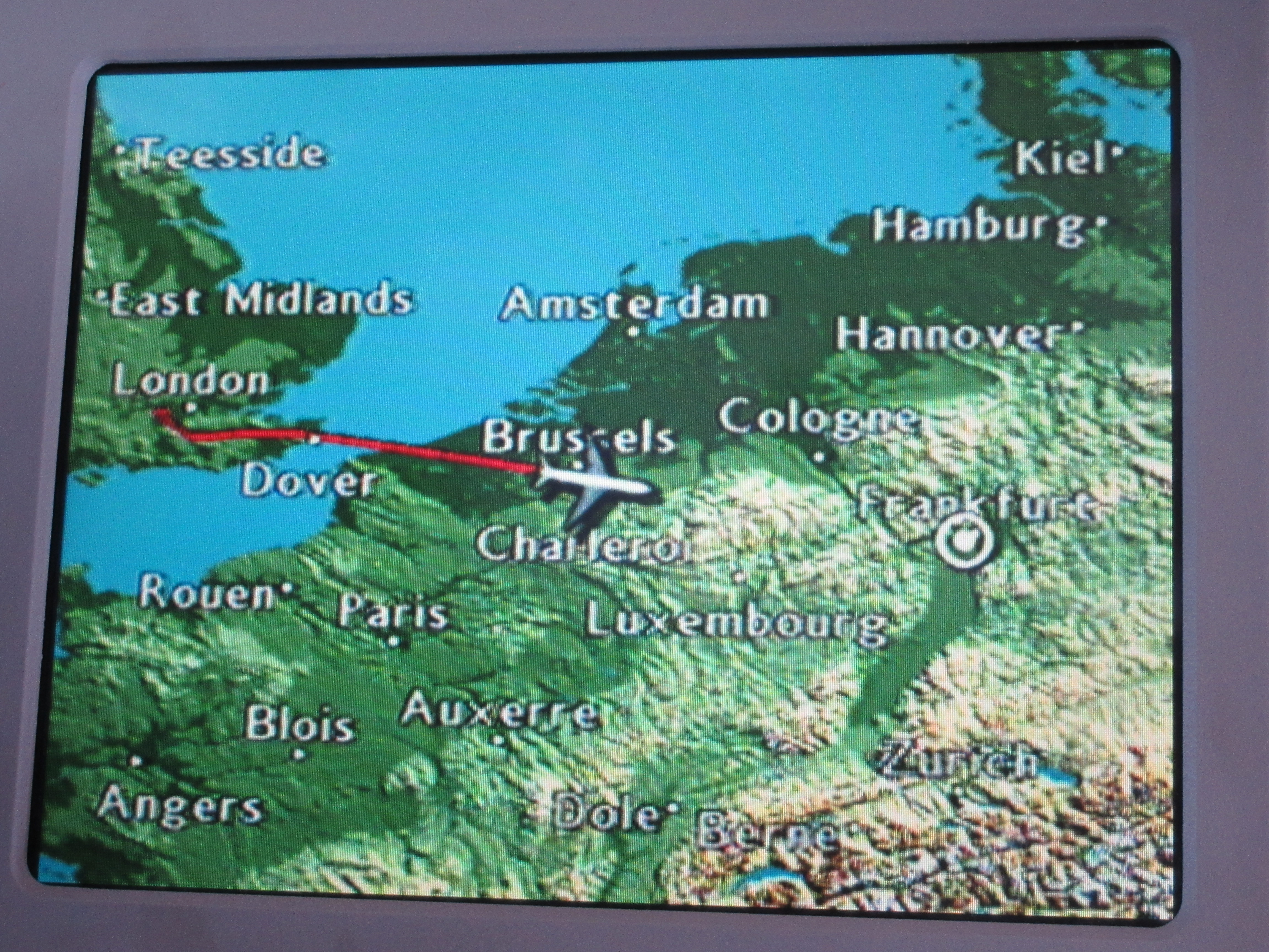
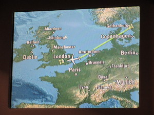
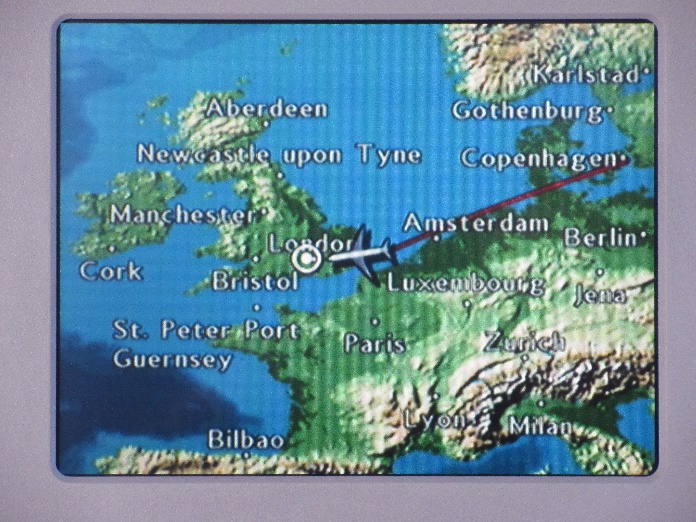
On Saturday afternoon we passed through London’s Heathrow airport for the third time in 5 days, this time continuing west to JFK, bringing the total for the week to 8,943km plus 300-odd in 3 different cars, 220 by rail, 25 by bus and 5 on the ferry 🙂 .
Sunday was spent with some of Dyalog’s North American contingent, co-ordinating and putting the final polish on the coming week’s presentations.
On Monday morning we were ready to start the first Dyalog North America user meeting – DYNA’15. The Princeton Crowne Plaza was our venue – making this our third time there after Dyalog ’07 and Dyalog ’09.
Back at the site of Dyalog ’07 and Dyalog ’09 – the Crowne Plaza in Princeton, New Jersey
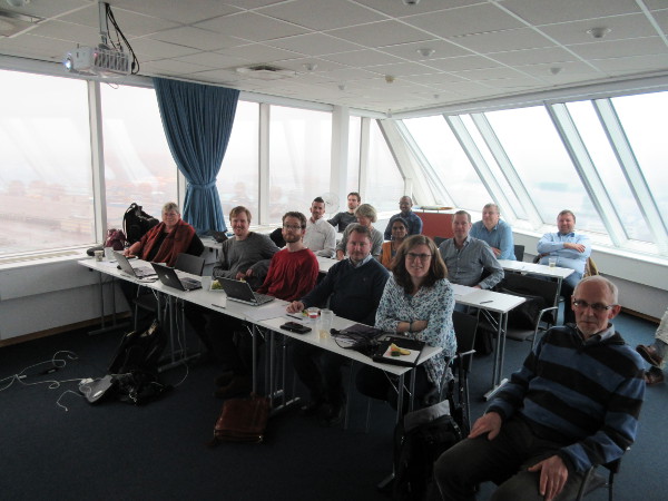
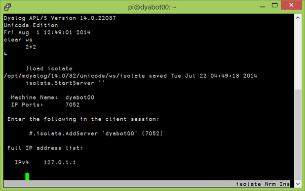
We had 37 visitors on Monday and 25 on Tuesday – a total of 45 different delegates representing about 15 different clients turned up to listen to updated road maps, demonstrations of new tools and four half-day workshops on Recent Language Enhancements, Parallel Programming using Futures and Isolates, Web Application Development and Modern APL Application Architectures. While there were no user presentations this year (the potential presenters seem to be keeping their powder dry for Dyalog ’15 in Sicily in September), we nonetheless had a full schedule.
Woodley Butler of Automatonics, Inc had been due to make a presentation, but had a scheduling problem and was unable to come. Gitte presented his exciting new hosting solution for Dyalog APL: APLCloud.com, during the opening session on Monday.
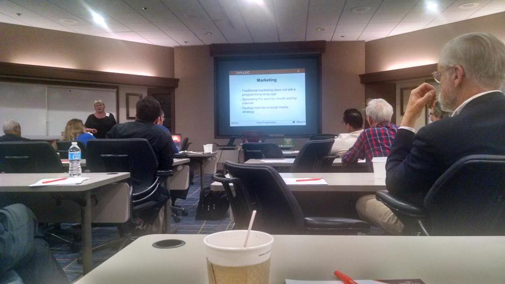
The view from the back – https://twitter.com/alexcweiner/status/590576821479067648/photo/1
Monday’s dinner may have been the highlight of the event. We traveled (longer than expected due to the shuttle driver getting lost) to Mimino’s Restaurant for an authentic Georgian meal. The word meal does not do the experience justice – it was a culinary extravaganza – with plate after plate of incredible Georgian food. Imagine everyone’s surprise when we were told that it was now time for the entrees! Good friends, good food and good drink made it a truly special night.
After a meeting in Princeton on Wednesday morning we hit the road, again, this time to the Poconos to spend a few days relaxing and working with the North American Dyaloggers on a variety of projects before wrapping this tour up with visits to clients next Monday and Tuesday.
 Follow