Welcome Ron Murray

Ron flying in 2003

Ron Murray is a recent addition to the Dyalog team, with a long history in the APL community. He first encountered APL/360 in 1969 and was hooked. He used it as the basis for teaching Computer Science courses for the Hampton, Virginia High Schools. Then, working with other APL pioneers, he wrote several APL applications and contributed to five different APL implementations at The Computer Company, STSC, Burroughs, Data Resources, and Analogic Corporation.

From 1986 until 2019 he left the world of APL to develop software on Microcomputers for Microsoft and Amazon, where he contributed to various development projects for Windows, OS/2, NT, Visual Basic, Encarta, and a variety of projects within the Microsoft Research Division as well the Developer Relations Group. He also contributed to the scalability and reliability of the Amazon transaction accounting system and the Windows Azure Archival Storage System.

He also ran an Aviation business for several years at the Tacoma Narrows airport, and started an internet television company with three friends. Together they learned a lot about crawling the web using machine learning, categorizing videos by their subject matters and quality, as well as constructing interactive user interfaces on IOS devices.

During all that non-APL work he continued to use APL as a tool of thought for organizing, analyzing, and clarifying the work that needed to be done.

Since July of 2020 he’s been applying the many non-APL things he’s learned to help extend and improve the Dyalog APL systems and their interactions with the rest of the computing world.

He points out that Windows 95, which is now 25 years old is about half as old as the APL/360 release!

Welcome Kirstine (Stine) Kromberg

Stine graduated from Copenhagen Business School with a Masters degree in Business Administration and Information Management in 2016, and went to work for a small consultancy firm. She started with “Drag&Drop” programming in SSIS and other similar tools, but quickly moved into project management, accounting, and Business Intelligence.

Covid-19 intervened just as she was looking forward to coming back from maternity leave, and she decided not to burden her previous employer by returning to a job as a consultant in a world where no-one really wanted external consultants for an unknown length of time. Since Dyalog was looking for a new accountant due to Helene’s retirement, she accepted that job. She hopes that she will soon have an opportunity to help the development team with project management as well.

If her last name sound somewhat familiar, it is because Stine is closely related to Gitte and Morten! Stine grew up in a household where APL was a part of everyday life. After swimming against the tide for many years she finally accepted a bet with Morten to give his “hobby” (APL) a try if he gave her hobby (Roleplaying) a try in return. As a result, she spent 2 weeks in Montreal trying to learn from one of the best teachers of APL. But while she learned a little French from staying at Dan Baronet’s house, the APL did not really stick. Morten sadly never got around to roleplaying, but he did take up Zumba many years later, so they consider the deal settled!

Several years later, while looking for something to do as a summer job, she took a job at Insight Systems learning APL while proofreading the new Dyalog APL book by Bernard Legrand and correcting data in the CRM system.

For several years she was hired to help run the help desk at the user meetings whenever they took place in Denmark. Her last appearance at a Dyalog user meeting was as a Zumba instructor in 2012 in Elsinore.

Stine has spent most of her life dancing around the edges of Dyalog, coming to the user meetings and chatting with customers and developers alike, hanging out at the office in Bramley, listening in whenever Gitte and Morten talked shop at the dinner table, trying to learn APL, but realizing that where her heart truly lies is in organizing and managing things. So, while working for an APL company feels like coming home, her ambition is not to take part in development, but instead to take care of all the details and bureaucracy so that the rest of our brilliant team can focus on what they truly love!

Warming up to Dyalog ’20 Online with the last Recording from Dyalog ’19!

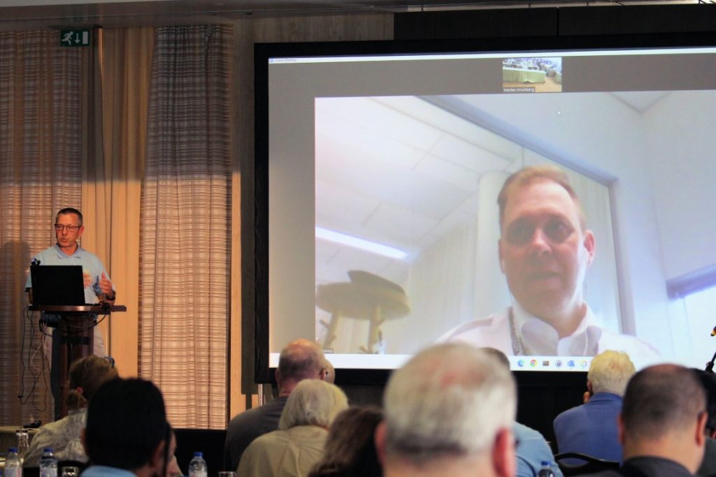
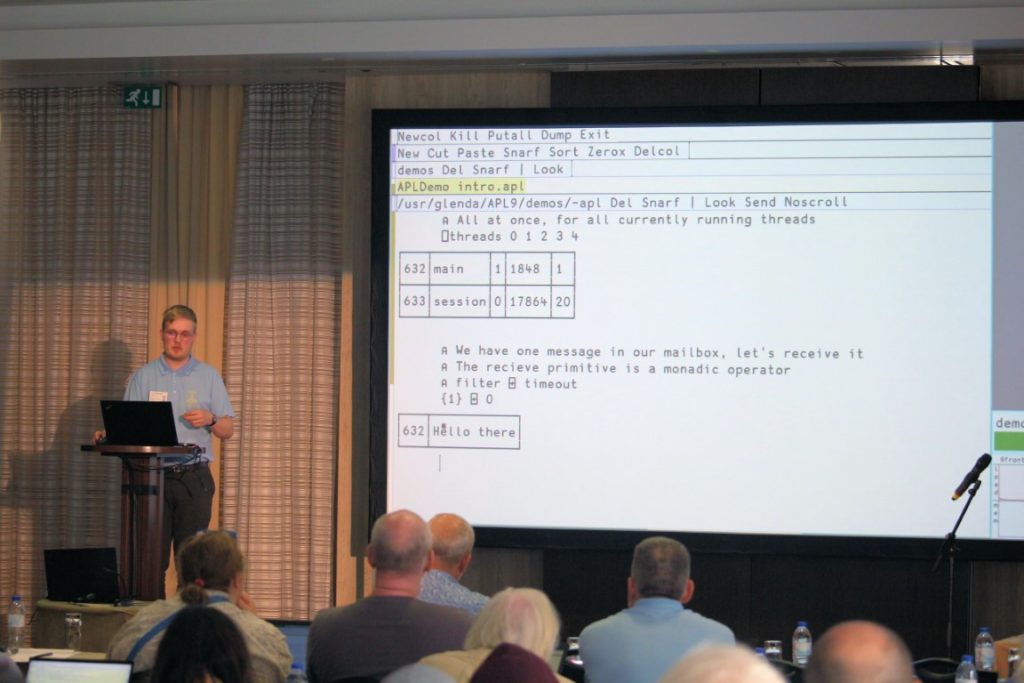
Three weeks from today, Gitte Christensen and I will be opening the 2020 Dyalog user meeting. Like so many similar gatherings, we are moving online; this year’s meeting will consist of two 4-hour sessions on Monday 9th and Tuesday 10th November, running from 14:00 to 18:00 UTC. Our hope (so far confirmed by advance registrations) is that this format will allow many more people to attend than a normal meeting, which requires you to set a full week aside and spend money on travel. We hope that the timing will allow attendance from a large part of the globe, and of course it is our intention to make recordings available afterwards for those unable to attend live.

I do subscribe to the proverb about all clouds having silver linings: although all the user meetings that I usually travel to attend have been cancelled or postponed, and I have missed meeting many of you face-to-face this year, it is important to note the unexpected side-effect; there is significantly more APL content being generated and made generally available than ever before! I hope that you have all noticed that Dyalog and the British APL Association have been holding online sessions every two weeks since the spring! A good place to keep track of these events is our event calendar at https://www.dyalog.com/dates-for-your-diary.htm.

Two four-hour sessions is obviously a lot less than the usual 3.5 days plus workshops. You should be able to find a good deal of the “missing” material, such as Adam Brudzewsky’s five-part series on features of Dyalog Version 18.0 (and my own introduction to the new release) at https://dyalog.tv/Webinar, where you can watch it at your leisure.

During Dyalog ’20 we will focus on giving you updates on the most important activities that the team behind Dyalog APL is currently working on. Also, although you may have to wait for Dyalog ’21 in Portugal to meet the winner of the APL Problem Solving Competition in person, Andrii Makukha from the University of Hong Kong will be giving his acceptance presentation online on the Tuesday. Chris and Michael Hughes will give us an update on a tool called qWC, which simplifies the transformation of existing Windows applications into web apps.

Calculating estimates for the paths of debris from M/S Irma.

Calculating estimates for the paths of debris from M/S Irma.

At Dyalog ’19, Tomas Gustafsson, author of the stunning Stormwind boat/ship simulator (real time physics engine implemented in Dyalog APL) told the story of the successful search for the M/S Irma, which was was lost in a sudden autumn storm between Finland and Sweden 50 years ago. Because a Finnish TV channel was producing a programme about the Irma, Tomas asked us not to publish the recording of his presentation last year. The embargo has finally been lifted, and we are now able to present the final recording from Dyalog ’19. In Tomas’ Dyalog ’19 video, you can hear Tomas tell the story of how, despite massive search efforts, said to be the biggest ever in Finnish history, the Irma accident became a mystery. No distress signals were heard during that fatal autumn night, and Irma had chosen the weirdest routes. Only one body was ever found, days later, at an unexpected location. Wreckage from the ship was discovered in the archipelago at multiple contradictory spots. Irma was found in May 2019 by a group of enthusiasts (including Tomas). The reverse drifting patterns calculated using Dyalog played a crucial role in the success of the search. Tomas will be back at Dyalog ’20 to entertain us with the story of his latest adventure: the search for a 500-year-old wreck, the Hanseatic hulk Hanneke Vrome, which left Lübeck at the brink of winter in 1468, to avoid Danish pirates.

I look forward to welcoming you to Dyalog ’20 on November 9th.

Towards Improvements to Stencil

Background

The stencil operator was introduced in Dyalog version 16.0 in 2017. Recently we received some feedback (OK, complaints) that (a) stencil does padding which is unwanted sometimes and needs to be removed from the result and (b) stencil is too slow when it is not supported by special code.

First, stencil in cases supported by special code is much faster than when it is not. The special cases are as follows, from Dyalog ’17 Workshop SA3.

   {⍵}      {⊢⍵}      {,⍵}      {⊂⍵}
{+/,⍵}    {∧/,⍵}    {∨/,⍵}    {=/,⍵}    {≠/,⍵}  
    
{  +/,A×⍵}    {  +/⍪A×⍤2⊢⍵}
{C<+/,A×⍵}    {C<+/⍪A×⍤2⊢⍵}
C:  a single number or variable whose value is a single number
A:  a variable whose value is a rank-2 or 3 array
The comparison can be < ≤ ≥ > = ≠
odd window size; movement 1; matrix argument
 

You can test whether a particular case is supported by using a circumlocution to defeat the special case recognizer.

   )copy dfns cmpx

   cmpx '{⍵}⌺3 5⊢y' '{⊢⊢⍵}⌺3 5⊢y' ⊣ y←?100 200⍴0
  {⍵}⌺3 5⊢x   → 4.22E¯4 |      0%                               
  {⊢⊢⍵}⌺3 5⊢x → 5.31E¯2 | +12477% ⎕⎕⎕⎕⎕⎕⎕⎕⎕⎕⎕⎕⎕⎕⎕⎕⎕⎕⎕⎕⎕⎕⎕⎕⎕⎕⎕⎕⎕⎕

   cmpx '{⌽⍵}⌺3 5⊢y' '{⊢⊢⌽⍵}⌺3 5⊢y'
  {⌽⍵}⌺3 5⊢y   → 2.17E¯1 |  0% ⎕⎕⎕⎕⎕⎕⎕⎕⎕⎕⎕⎕⎕⎕⎕⎕⎕⎕⎕⎕⎕⎕⎕⎕⎕⎕⎕⎕⎕⎕
  {⊢⊢⌽⍵}⌺3 5⊢y → 2.21E¯1 | +1% ⎕⎕⎕⎕⎕⎕⎕⎕⎕⎕⎕⎕⎕⎕⎕⎕⎕⎕⎕⎕⎕⎕⎕⎕⎕⎕⎕⎕⎕⎕

If the timings are the same then there is no special code.

Padding and performance improvements will take a lot of work. For example, for padding (i.e. the treatment of cells at the edge of the universe) multiple options are possible: no padding, padding, wrap from opposite edge, etc. While working on these improvements I hit upon the idea of writing a stencil function which produces the stencil cells. It only works with no padding and only for movements of 1 (which I understand are common cases), but turns out to be an interesting study.

A Stencil Function

⍺ stencell ⍵ produces the stencil cells of size from  , and is equivalent to {⍵}⌺⍺⊢⍵ after the padded cells are removed.

stencell←{
  ⎕io←0                 ⍝ ⎕io delenda est!
  s←(≢⍺)↑⍴⍵
  f←1+s-⍺               ⍝ frame AKA outer shape
  m←⊖×⍀⊖1↓s,1           ⍝ multiplier for each axis
  i←⊃∘.+⌿(m,m)×⍳¨f,⍺    ⍝ indices
  (⊂i) ⌷ ⍵ ⍴⍨ (×⌿(≢⍺)↑⍴⍵),(≢⍺)↓⍴⍵
}

For example, stencell is applied to x with cell shape 3 5 .

   ⊢ x←6 10⍴⍳60                    ⍝ (a)
 0  1  2  3  4  5  6  7  8  9
10 11 12 13 14 15 16 17 18 19
20 21 22 23 24 25 26 27 28 29
30 31 32 33 34 35 36 37 38 39
40 41 42 43 44 45 46 47 48 49
50 51 52 53 54 55 56 57 58 59

   c←3 5 stencell x                ⍝ (b)
   ⍴c
4 6 3 5

   c ≡ 1 2 ↓ ¯1 ¯2 ↓ {⍵}⌺3 5 ⊢x    ⍝ (c)
1

   ⊢ e←⊂⍤2 ⊢c                      ⍝ (d)
┌──────────────┬──────────────┬──────────────┬──────────────┬──────────────┬──────────────┐
│ 0  1  2  3  4│ 1  2  3  4  5│ 2  3  4  5  6│ 3  4  5  6  7│ 4  5  6  7  8│ 5  6  7  8  9│
│10 11 12 13 14│11 12 13 14 15│12 13 14 15 16│13 14 15 16 17│14 15 16 17 18│15 16 17 18 19│
│20 21 22 23 24│21 22 23 24 25│22 23 24 25 26│23 24 25 26 27│24 25 26 27 28│25 26 27 28 29│
├──────────────┼──────────────┼──────────────┼──────────────┼──────────────┼──────────────┤
│10 11 12 13 14│11 12 13 14 15│12 13 14 15 16│13 14 15 16 17│14 15 16 17 18│15 16 17 18 19│
│20 21 22 23 24│21 22 23 24 25│22 23 24 25 26│23 24 25 26 27│24 25 26 27 28│25 26 27 28 29│
│30 31 32 33 34│31 32 33 34 35│32 33 34 35 36│33 34 35 36 37│34 35 36 37 38│35 36 37 38 39│
├──────────────┼──────────────┼──────────────┼──────────────┼──────────────┼──────────────┤
│20 21 22 23 24│21 22 23 24 25│22 23 24 25 26│23 24 25 26 27│24 25 26 27 28│25 26 27 28 29│
│30 31 32 33 34│31 32 33 34 35│32 33 34 35 36│33 34 35 36 37│34 35 36 37 38│35 36 37 38 39│
│40 41 42 43 44│41 42 43 44 45│42 43 44 45 46│43 44 45 46 47│44 45 46 47 48│45 46 47 48 49│
├──────────────┼──────────────┼──────────────┼──────────────┼──────────────┼──────────────┤
│30 31 32 33 34│31 32 33 34 35│32 33 34 35 36│33 34 35 36 37│34 35 36 37 38│35 36 37 38 39│
│40 41 42 43 44│41 42 43 44 45│42 43 44 45 46│43 44 45 46 47│44 45 46 47 48│45 46 47 48 49│
│50 51 52 53 54│51 52 53 54 55│52 53 54 55 56│53 54 55 56 57│54 55 56 57 58│55 56 57 58 59│
└──────────────┴──────────────┴──────────────┴──────────────┴──────────────┴──────────────┘

    ∪¨ ,¨ e-⍬⍴e                    ⍝ (e)
┌──┬──┬──┬──┬──┬──┐
│0 │1 │2 │3 │4 │5 │
├──┼──┼──┼──┼──┼──┤
│10│11│12│13│14│15│
├──┼──┼──┼──┼──┼──┤
│20│21│22│23│24│25│
├──┼──┼──┼──┼──┼──┤
│30│31│32│33│34│35│
└──┴──┴──┴──┴──┴──┘
(a)  The matrix x is chosen to make stencil results easier to understand.
(b) stencell is applied to x with cell shape 3 5 .
(c) The result of stencell is the same as that for {⍵}⌺ after cells with padding are dropped.
(d) Enclose the matrices in c (the cells) to make the display more compact and easier to understand.
(e) Subsequent discussion is based on the observation that each cell is some scalar integer added to the first cell.

Indices

The key expression in the computation is

   ⊃∘.+⌿(m,m)×⍳¨f,⍺ 

where

   m:  10 1;  multiplier for each axis
   f:  4 6;  multiplier for each axis
   ⍺:  3 5;  multiplier for each axis
 

We discuss a more verbose but equivalent version of this expression,

   (⊃∘.+⌿m×⍳¨f)∘.+(⊃∘.+⌿m×⍳¨⍺)

and in particular the right half, ⊃∘.+⌿m×⍳¨⍺ , which produces the first cell.

   ⍳⍺               ⍝ ⍳3 5
┌───┬───┬───┬───┬───┐
│0 0│0 1│0 2│0 3│0 4│
├───┼───┼───┼───┼───┤
│1 0│1 1│1 2│1 3│1 4│
├───┼───┼───┼───┼───┤
│2 0│2 1│2 2│2 3│2 4│
└───┴───┴───┴───┴───┘
   (⍴⍵)∘⊥¨⍳⍺        ⍝ 6 10∘⊥¨ ⍳3 5
 0  1  2  3  4
10 11 12 13 14
20 21 22 23 24

Alternatively, this last result obtains by multiplying by m the corresponding indices for each axis, where an element of m is the increment for a unit in an axis. That is, m←⊖×⍀⊖1↓s,1 where s←(≢⍺)↑⍴⍵ is a prefix of the shape of  . The multipliers are with respect to the argument because the indices are required to be with respect to the argument  .

   ⍳¨⍺              ⍝ ⍳¨3 5
┌─────┬─────────┐
│0 1 2│0 1 2 3 4│
└─────┴─────────┘
   m×⍳¨⍺            ⍝ 10 1×⍳¨3 5
┌───────┬─────────┐
│0 10 20│0 1 2 3 4│
└───────┴─────────┘
   ∘.+⌿ m×⍳¨⍺       ⍝ ∘.+⌿ 10 1×⍳¨3 5
┌──────────────┐
│ 0  1  2  3  4│
│10 11 12 13 14│
│20 21 22 23 24│
└──────────────┘
   ((⍴⍵)∘⊥¨⍳⍺) ≡ ⊃∘.+⌿m×⍳¨⍺
1

This alternative computation is more efficient because it avoids creating and working on lots of small nested vectors and because the intermediate results for ∘.+⌿ grows fast from one to the next (i.e., O(⍟n) iterations in the main loop).

The left half, ⊃∘.+⌿m×⍳¨f , is similar, and computes the necessary scalar integers to be added to the result of the right half.

   ⊃ ∘.+⌿ m×⍳¨f     ⍝ ⊃ ∘.+⌿ 10 1×⍳¨4 6
 0  1  2  3  4  5
10 11 12 13 14 15
20 21 22 23 24 25
30 31 32 33 34 35

The shorter expression derives from the more verbose one by some simple algebra.

(⊃∘.+⌿m×⍳¨f)∘.+(⊃∘.+⌿m×⍳¨⍺)    ⍝ verbose version
⊃∘.+⌿(m×⍳¨f),m×⍳¨⍺             ⍝ ∘.+ is associative
⊃∘.+⌿(m,m)×(⍳¨f),⍳¨⍺           ⍝ m× distributes over ,
⊃∘.+⌿(m,m)×⍳¨f,⍺               ⍝ ⍳¨ distributes over ,

I am actually disappointed that the shorter expression was found ☺; it would have been amusing to have a non-contrived and short expression with three uses of ∘.+ .

Cells

Having the indices i in hand, the stencil cells obtain by indexing into an appropriate reshape or ravel of the right argument  . In general, the expression is

   (⊂i) ⌷ ⍵ ⍴⍨ (×/(≢⍺)↑⍴⍵),(≢⍺)↓⍴⍵

specifies the cell shape. If (≢⍺)=≢⍴⍵ , that is, if a length is specified for each axis of  , the expression is equivalent to (⊂i)⌷,⍵ or (,⍵)[i] ; if (≢⍺)<≢⍴⍵ , that is, if there are some trailing unstencilled axes, the expression is equivalent to (,[⍳≢⍺]⍵)[i;…;] (the leading ≢⍺ axes are ravelled) or ↑(,⊂⍤((≢⍴⍵)-≢⍺)⊢⍵)[i] (as if the trailing axes were shielded from indexing). The general expression covers both cases.

Application

stencell makes it possible to workaround current shortcomings in . The alternative approach is to use stencell to get all the stencil cells, all at once, and then work on the cells using  , +.× , and
other efficient primitives.

The following example is from Aaron Hsu. In the original problem the size of x is 512 512 64 .

   K←?64 3 3 64⍴0
   x←?256 256 64⍴0

   t←1 1↓¯1 ¯1↓{+/⍪K×⍤3⊢⍵}⌺3 3⊢x
   ⍴t
256 256 64

   cmpx '1 1↓¯1 ¯1↓{+/⍪K×⍤3⊢⍵}⌺3 3⊢x'
6.76E0 

The computation is slow because the cells are rank-3, not supported by special code. Aaron then devised a significant speed-up using a simpler left operand to create the ravels of the cells (but still no special code):

   t ≡ (1 1↓¯1 ¯1↓{,⍵}⌺3 3⊢x)+.×⍉⍪K
1
   cmpx '(1 1↓¯1 ¯1↓{,⍵}⌺3 3⊢x)+.×⍉⍪K'
1.67E0 

Use of stencell would improve the performance a bit further:

   t ≡ (,⍤3 ⊢3 3 stencell x)+.×⍉⍪K
1
   cmpx '(,⍤3 ⊢3 3 stencell x)+.×⍉⍪K'
1.09E0 

   cmpx '3 3 stencell x'
6.10E¯2

The last timing shows that the stencell computation is 6% (6.10e¯2÷1.09e0) of the total time.

Materializing all the cells does take more space than if the computation is incorporated in the left operand of  , and is practicable only if the workspace sufficiently large.

   )copy dfns wsreq

   wsreq '1 1↓¯1 ¯1↓{+/⍪K×⍤3⊢⍵}⌺3 3⊢x'
110649900
   wsreq '(1 1↓¯1 ¯1↓{,⍵}⌺3 3⊢x)+.×⍉⍪K'
647815900
   wsreq '(,⍤3 ⊢3 3 stencell x)+.×⍉⍪K'
333462260

Performance

stencell is competitive with {⍵}⌺ on matrices, where it is supported by special code written in C, and is faster when there is no special code. The benchmarks are done on a larger argument to reduce the effects of padding/unpadding done in {⍵}⌺ .

   y2←?200 300⍴0
          
   cmpx '3 5 stencell y2' '1 2↓¯1 ¯2↓{⍵}⌺3 5⊢y2' 
  3 5 stencell y      → 1.85E¯3 |   0% ⎕⎕⎕⎕⎕⎕⎕⎕⎕⎕⎕⎕⎕⎕⎕⎕⎕⎕⎕           
  1 2↓¯1 ¯2↓{⍵}⌺3 5⊢y → 2.91E¯3 | +57% ⎕⎕⎕⎕⎕⎕⎕⎕⎕⎕⎕⎕⎕⎕⎕⎕⎕⎕⎕⎕⎕⎕⎕⎕⎕⎕⎕⎕⎕⎕

   cmpx '3 5 stencell y' '{⍵}⌺3 5⊢y' 
  3 5 stencell y → 1.85E¯3 |   0% ⎕⎕⎕⎕⎕⎕⎕⎕⎕⎕⎕⎕⎕⎕⎕⎕⎕⎕⎕⎕⎕⎕⎕⎕⎕⎕⎕⎕⎕⎕
* {⍵}⌺3 5⊢y      → 1.04E¯3 | -45% ⎕⎕⎕⎕⎕⎕⎕⎕⎕⎕⎕⎕⎕⎕⎕⎕⎕             

   y3←?200 300 64⍴0

   cmpx '3 5 stencell y3' '1 2↓¯1 ¯2↓{⍵}⌺3 5⊢y3' 
  3 5 stencell y3      → 8.90E¯2 |    0% ⎕⎕⎕                           
  1 2↓¯1 ¯2↓{⍵}⌺3 5⊢y3 → 7.78E¯1 | +773% ⎕⎕⎕⎕⎕⎕⎕⎕⎕⎕⎕⎕⎕⎕⎕⎕⎕⎕⎕⎕⎕⎕⎕⎕⎕⎕⎕⎕⎕⎕

   cmpx '3 5 stencell y3' '{⍵}⌺3 5⊢y3' 
  3 5 stencell y3 → 9.38E¯2 |    0% ⎕⎕⎕⎕⎕⎕⎕⎕                      
* {⍵}⌺3 5⊢y3      → 3.34E¯1 | +256% ⎕⎕⎕⎕⎕⎕⎕⎕⎕⎕⎕⎕⎕⎕⎕⎕⎕⎕⎕⎕⎕⎕⎕⎕⎕⎕⎕⎕⎕⎕

There is an interesting question of whether the shorter version of the key computation (in the Indices section above) is faster than the more verbose version.

   m←10 1 ⋄ f←4 6 ⋄ a←3 5

   cmpx '⊃∘.+⌿(m,m)×⍳¨f,a' '(⊃∘.+⌿m×⍳¨f)∘.+(⊃∘.+⌿m×⍳¨a)'
  ⊃∘.+⌿(m,m)×⍳¨f,a            → 3.75E¯6 |   0% ⎕⎕⎕⎕⎕⎕⎕⎕⎕⎕⎕⎕⎕⎕⎕⎕⎕⎕⎕
  (⊃∘.+⌿m×⍳¨f)∘.+(⊃∘.+⌿m×⍳¨a) → 5.20E¯6 | +38% ⎕⎕⎕⎕⎕⎕⎕⎕⎕⎕⎕⎕⎕⎕⎕⎕⎕⎕⎕⎕⎕⎕⎕⎕⎕⎕

In this case, it is faster, and I expect it will be faster for cases which arise in stencil calculations, where the argument size is larger than the cell size. But it is easy to think of arguments where ∘.+⌿ is slower than ∘.+ done with a different grouping:

   cmpx '((⍳0)∘.+⍳100)∘.+⍳200' '(⍳0)∘.+((⍳100)∘.+⍳200)' '⊃∘.+/⍳¨0 100 200'
  ((⍳0)∘.+⍳100)∘.+⍳200   → 7.86E¯7 |     0% ⎕⎕                            
  (⍳0)∘.+((⍳100)∘.+⍳200) → 1.05E¯5 | +1234% ⎕⎕⎕⎕⎕⎕⎕⎕⎕⎕⎕⎕⎕⎕⎕⎕⎕⎕⎕⎕⎕⎕⎕⎕⎕⎕⎕⎕  
  ⊃∘.+/⍳¨0 100 200       → 1.11E¯5 | +1310% ⎕⎕⎕⎕⎕⎕⎕⎕⎕⎕⎕⎕⎕⎕⎕⎕⎕⎕⎕⎕⎕⎕⎕⎕⎕⎕⎕⎕⎕⎕

This question will be explored further in a later post.

2019 APL Problem Solving Competition: Phase I Problems Sample Solutions

The following are my attempts at the Phase I problems of the 2019 APL Problem Solving Competition. There are not necessarily “right answers” as personal style and taste come into play. More explanation of the code is provided here than common practice. All solutions pass all the tests specified in the official problem description.

1. Chunky Monkey

Write a function that, given a scalar or vector as the right argument and a positive (>0) integer chunk size n as the left argument, breaks the array’s items up into chunks of size n. If the number of elements in the array is not evenly divisible by n, then the last chunk will have fewer than n elements.

💡Hint: The partitioned enclose function could be helpful for this problem.

   f1←{((≢⍵)⍴⍺↑1)⊂⍵}

Basically, the problem is to construct an appropriate boolean left argument to. For this the reshape function ⍺⍴⍵ is apt, which repeats the items of up to length .

   9 ⍴ 1 0 0                     (9 ⍴ 1 0 0) ⊂ 'ABCDEFGHI'
1 0 0 1 0 0 1 0 0             ┌───┬───┬───┐
                              │ABC│DEF│GHI│
                              └───┴───┴───┘

   11 ⍴ 1 0 0                    (11 ⍴ 1 0 0) ⊂ 'ABCDEFGHIJK'
1 0 0 1 0 0 1 0 0 1 0         ┌───┬───┬───┬──┐
                              │ABC│DEF│GHI│JK│
                              └───┴───┴───┴──┘

2. Making the Grade

Score Range Letter Grade
0-64 F
65-69 D
70-79 C
80-89 B
90-100 A
 

Write a function that, given an array of integer test scores in the inclusive range 0–100, returns an identically-shaped array of the corresponding letter grades according to the table to the left.

💡Hint: You may want to investigate the interval index function.

   f2← {'FDCBA'[0 65 70 80 90⍸⍵]}

For example:

   range← 0 65 70 80 90
   score← 0 65 89 64 75 100

   range ⍸ score                      range ⍸ 2 3⍴score
1 2 4 1 3 5                        1 2 4
                                   1 3 5
   'FDCBA'[1 2 4 1 3 5]               'FDCBA'[2 3⍴1 2 4 1 3 5]
FDBFCA                             FDB
                                   FCA
    f2 score                          f2 2 3⍴score
FDBFCA                             FDB
                                   FCA

The examples on the right illustrate that the functionsand [] extend consistently to array arguments.

In APL, functions take array arguments, and so too indexing takes array arguments, including the indices (the “subscripts”). This property is integral to the template

   Y indexing (X index ⍵)

where

 
X   domain for looking things up
Y range where you want to end up; “aliases” corresponding to X
index a function to do the looking up, such asor
indexing   a function to do indexing into X , such as [] or or (dyadic)

3. Grade Distribution

Given a non-empty character vector of single-letter grades, produce a 3-column, 5-row, alphabetically-sorted matrix of each grade, the number of occurrences of that grade, and the percentage (rounded to 1 decimal position) of the total number of occurrences of that grade. The table should have a row for each grade even if there are no occurrences of a grade. Note: due to rounding the last column might not total 100%.

💡Hint: The key operator could be useful for this problem.

   f3←{a,k,1⍕⍪100×k÷+⌿k←¯1+{≢⍵}⌸⍵⍪⍨a←'ABCDF'}

The result of f⌸ is ordered by the unique major cells in the keys. If a particular order is required, or if a particular set of keys is required (even when some keys don’t occur in the argument), the computation can be effected by prefacing keys to the argument (here ,⍨a←'ABCDF') and then applying an inverse function (here ¯1+) to the result of .

For the key operator, in particular cases, for example the letter distribution in a corpus of English text, the universe of letters and their ordering are known (A-Z); in principle, it is not possible to “know” the complete universe of keys, or their ordering.

The function f3x illustrates the complications. f3 is the same as above; extra spaces are inserted into both functions to facilitate comparison.

   f3 ← {a,   k,1⍕⍪100×k÷+⌿k←¯1+{≢⍵}⌸⍵⍪⍨a←'ABCDF'}
   f3x← {(∪⍵),k,1⍕⍪100×k÷+⌿k←   {≢⍵}⌸⍵           }

   ⊢ g1← 9 3 8 4 7/'DABFC'
DDDDDDDDDAAABBBBBBBBFFFFCCCCCCC

   f3x g1                            f3 g1
D 9  29.0                         A 3   9.7
A 3   9.7                         B 8  25.8
B 8  25.8                         C 7  22.6
F 4  12.9                         D 9  29.0
C 7  22.6                         F 4  12.9
                  
   ⊢ g2← ('F'≠grade)⌿grade
DDDDDDDDDAAABBBBBBBBCCCCCCC

   f3x g2                            f3 g2
D 9  33.3                         A 3  11.1
A 3  11.1                         B 8  29.6
B 8  29.6                         C 7  25.9
C 7  25.9                         D 9  33.3
                                  F 0   0.0

4. Knight Moves

┌───┬───┬───┬───┬───┬───┬───┬───┐
│1 1│1 2│1 3│1 4│1 5│1 6│1 7│1 8│
├───┼───┼───┼───┼───┼───┼───┼───┤
│2 1│2 2│2 3│2 4│2 5│2 6│2 7│2 8│
├───┼───┼───┼───┼───┼───┼───┼───┤
│3 1│3 2│3 3│3 4│3 5│3 6│3 7│3 8│
├───┼───┼───┼───┼───┼───┼───┼───┤
│4 1│4 2│4 3│4 4│4 5│4 6│4 7│4 8│
├───┼───┼───┼───┼───┼───┼───┼───┤
│5 1│5 2│5 3│5 4│5 5│5 6│5 7│5 8│
├───┼───┼───┼───┼───┼───┼───┼───┤
│6 1│6 2│6 3│6 4│6 5│6 6│6 7│6 8│
├───┼───┼───┼───┼───┼───┼───┼───┤
│7 1│7 2│7 3│7 4│7 5│7 6│7 7│7 8│
├───┼───┼───┼───┼───┼───┼───┼───┤
│8 1│8 2│8 3│8 4│8 5│8 6│8 7│8 8│
└───┴───┴───┴───┴───┴───┴───┴───┘
  Consider a chess board as an 8×8 matrix with square (1 1) in the upper left corner and square (8 8) in the lower right corner. For those not familiar with the game a chess, the knight, generally depicted as a horse (♞), can move 2 spaces right or left and then 1 space up or down, or 2 spaces up or down and then 1 space right or left. For example, this means that a knight on the square (5 4) can move to any of the underscored squares.

Given a 2-element vector representing the current square for a knight, return a vector of 2-element vectors representing (in any order) all the squares that the knight can move to.

💡Hint: The outer product operator ∘. could be useful for generating the coordinates.

   f4← {↓(∧/q∊⍳8)⌿q←⍵+⍤1⊢(3=+/|t)⌿t←↑,∘.,⍨¯2 ¯1 1 2}

f4 derives as follows: First, generate all 16 combinations t of moves involving 1 and 2 steps, left and right and up and down, then select move combinations which total exactly 3 squares regardless of direction.

   (3=+/|t)⌿t←↑,∘.,⍨¯2 ¯1 1 2
¯2 ¯1
¯2  1
¯1 ¯2
¯1  2
 1 ¯2
 1  2
 2 ¯1
 2  1

The resultant 8-row matrix (call this mv) is added to, the coordinates of the current square, and then pruned to discard squares which fall outside of the chess board. The following examples illustrate the computation for ⍵≡5 4 and ⍵≡1 2 :

   mv←(3=+/|t)⌿t←↑,∘.,⍨¯2 ¯1 1 2

   ⊢ q←5 4+⍤1⊢mv                             ⊢ q←1 2+⍤1⊢mv
3 3                                       ¯1 1
3 5                                       ¯1 3
4 2                                        0 0
4 6                                        0 4
6 2                                        2 0
6 6                                        2 4
7 3                                        3 1
7 5                                        3 3

   ↓(∧/q∊⍳8)⌿q                               ↓(∧/q∊⍳8)⌿q
┌───┬───┬───┬───┬───┬───┬───┬───┐         ┌───┬───┬───┐
│3 3│3 5│4 2│4 6│6 2│6 6│7 3│7 5│         │2 4│3 1│3 3│
└───┴───┴───┴───┴───┴───┴───┴───┘         └───┴───┴───┘

An alterative solution is to precomputing an 8×8 table of the possible knight moves for each chess square, and then picking from the table:

   f4i← (f4¨ ⍳8 8) ⊃⍨ ⊂

The table look-up version would be more efficient in situations (such as in the Knight’s Tour puzzle) where the knight moves are computed repeatedly.
 

5. Doubling Up

Given a word or a list of words, return a Boolean vector where 1 indicates a word with one or more consecutive duplicated, case-sensitive, letters. Each word will have at least one letter and will consist entirely of either uppercase (A-Z) or lowercase (a-z) letters. Words consisting of a single letter can be scalars.

💡Hint: The nest functioncould be useful.

   f5← (∨⌿2=⌿' ',⊢)¨∘⊆

A solution obtains by solving it for one word and then applying it to each word via the each operator. Since a single word argument can be a string of letters, and we don’t want to apply the single word solution to each letter, that argument must first be converted in an enclosed word with nest. Thus the overall solution is of the form f¨∘⊆.

For a single word, what is required is to detect consecutive duplicate letters, whence the operator 2=⌿⍵ is apt.

   2 =⌿ 'bookkeeper'                  2 =⌿ 'radar'
0 1 0 1 0 1 0 0 0                  0 0 0 0

   ∨⌿ 2 =⌿ 'bookkeeper'               ∨⌿ 2 =⌿ 'radar'
1                                  0

As usual, the link function {⍺⍵} can be used as a generic dyadic operand function to gain additional insight into the workings of an operator:

   2 {⍺⍵}⌿ 'bookkeeper'               2 {⍺⍵}⌿ 'radar'
┌──┬──┬──┬──┬──┬──┬──┬──┬──┐       ┌──┬──┬──┬──┐
│bo│oo│ok│kk│ke│ee│ep│pe│er│       │ra│ad│da│ar│
└──┴──┴──┴──┴──┴──┴──┴──┴──┘       └──┴──┴──┴──┘

2 f⌿⍵ signals error on single-item arguments; moreover, it is problematic to compare a single letter against itself. Both problems are finessed by first prefacing the argument with a space ' '.

In f5, the train (∨⌿2=⌿' ',⊢) can also be written as the equivalent dfn {∨⌿2=⌿' ',⍵} as a matter of personal style. The display of a train does provide more information about how it is structured than the display of a dfn.

   (∨⌿2=⌿' ',⊢)                       {∨/2=⌿' ',⍵}
┌─────┬─────────────────┐          {∨⌿2=⌿' ',⍵}
│┌─┬─┐│┌─┬─────┬───────┐│
││∨│⌿│││2│┌─┬─┐│┌─┬─┬─┐││
│└─┴─┘││ ││=│⌿│││ │,│⊢│││
│     ││ │└─┴─┘│└─┴─┴─┘││
│     │└─┴─────┴───────┘│
└─────┴─────────────────┘

6. Telephone Names

┌────┬───┬────┐
│    │ABC│DEF │
│ 1  │ 2 │ 3  │
├────┼───┼────┤
│GHI │JKL│MNO │
│ 4  │ 5 │ 6  │
├────┼───┼────┤
│PQRS│TUV│WXYZ│
│ 7  │ 8 │ 9  │
├────┼───┼────┤
│    │   │    │
│ *  │ 0 │ #  │
└────┴───┴────┘
  Some telephone keypads have letters of the alphabet embossed on their keytops. Some people like to remember phone numbers by converting them to an alphanumeric form using one of the letters on the corresponding key. For example, in the keypad shown, 'ALSMITH' would correspond to the number 257-6484 and '1DYALOGBEST' would correspond to 1-392-564-2378. Write an APL function that takes a character vector right argument that consists of digits and uppercase letters and returns an integer vector of the corresponding digits on the keypad.

💡Hint: Your solution might make use of the membership function .

   f6← {(⍵⍸⍨⎕d,'ADGJMPTW')-9*⍵∊⎕a}

Letters and digits alike are mapped to integer indices using the interval index function, which neatly handles the irregularly-sized intervals (see problem 2 above). The indices are then decremented by 9 for letters and by 1 for digits.

The expression 9*⍵∊⎕a illustrates a common technique in APL used to implement array logic, effecting control flow without using control structures or explicit branching. In the following, c and d are scalars (usually numbers) and is a boolean array.

c*⍵ c whereis 1 and 1 whereis 0.
c×⍵ c whereis 1 and 0 whereis 0.
c+⍵×d-c   c whereis 0 and d whereis 1.
(c,d)[1+⍵]   Same as c+⍵×d-c, but c and d can be any scalars. The 1+ is omitted if the index origin ⎕io is 0.

7. In the Center of It All

Given a right argument of a list of words (or possibly a single word) and a left argument of a width, return a character matrix that has width columns and one row per word, with each word is centered within the row. If width is smaller than the length of a word, truncate the word from the right. If there are an odd number of spaces to center within, leave the extra space on the right.

💡Hint: The mixand rotatefunctions will probably be useful here.

   f7← {(⌈¯0.5×0⌈⍺-≢¨⍵)⌽↑⍺↑¨⍵}∘⊆

As in problem 5, a prefatory application of nestconverts an argument of a single word into a more manageable standard of a list of words. Subsequently, the right argument is turned into a matrix, each row padded with spaces on the right (or truncated). Each row is then rotated so that the non-blank characters are centered. The finicky detail of an odd number of spaces is resolved by usingorin the calculation of the amounts of rotation.

8. Going the Distance

Given a vector of (X Y) points, or a single X Y point, determine the total distance covered when travelling in a straight line from the first point to the next one, and so on until the last point, then returning directly back to the start. For example, given the points

   (A B C)← (¯1.5 ¯1.5) (1.5 2.5) (1.5 ¯1.5)

the distance A to B is 5, B to C is 4 and C back to A is 3, for a total of 12.

💡Hint: The rotateand power * functions might be useful.

   f8← {+⌿ 2 {0.5*⍨+.×⍨⍺-⍵}⌿ ⍵⍪1↑⍵}

The result obtains by applying the distance function d←{0.5*⍨+.×⍨⍺-⍵} between pairs of points, taking care to return to the start.

As in problem 5, the expression 2 f⌿⍵ is just the ticket for working with consecutive items in the argument and, again, using the link function {⍺⍵} elucidates the workings of an operator:

   (A B C)← (¯1.5 ¯1.5) (1.5 2.5) (1.5 ¯1.5)

   2 {⍺⍵}⌿ A B C A
┌───────────────────┬──────────────────┬────────────────────┐
│┌─────────┬───────┐│┌───────┬────────┐│┌────────┬─────────┐│
││¯1.5 ¯1.5│1.5 2.5│││1.5 2.5│1.5 ¯1.5│││1.5 ¯1.5│¯1.5 ¯1.5││
│└─────────┴───────┘│└───────┴────────┘│└────────┴─────────┘│
└───────────────────┴──────────────────┴────────────────────┘
   2 d⌿ A B C A
5 4 3

   A d B              B d C              C d A
5                  4                   3

   f8 A B C
12

9. Area Code à la Gauss

Gauss’s area formula, also known as the shoelace formula, is an algorithm to calculate the area of a simple polygon (a polygon that does not intersect itself). It’s called the shoelace formula because of a common method using matrices to evaluate it. For example, the area of the triangle described by the vertices (2 4) (3 ¯8) (1 2) can be calculated by “walking around” the perimeter back to the first vertex, then drawing diagonals between the columns. The pattern created by the intersecting diagonals resembles shoelaces, hence the name “shoelace formula”.

💡Hint: You may want to investigate the rotate firstfunction.

First place the vertices in order above each other:
2 4
3 ¯8
1 2
2 4
Sum the products of the numbers connected by the diagonal lines going down and to the right:

      (2ׯ8)+(3×2)+(1×4)
¯6
      
2 4
3 ¯8
1 2
2 4
Next sum the products of the numbers connected by the diagonal lines going down and to the left:

      (4×3)+(¯8×1)+(2×2)
8
      
2 4
3 ¯8
1 2
2 4

Finally, halve the absolute value of the difference between the two sums:

      0.5 × | ¯6 - 8
7
      
2 4
3 ¯8
1 2
2 4

Given a vector of (X Y) points, or a single X Y point, return a number indicating the area circumscribed by the points.

   f9← {0.5×|(+/×/¯1↓0 1⊖t)-+/×/1↓0 ¯1⊖t←↑(⊢,1∘↑)⊆⍵}

There is an alternative solution using the determinant function and the stencil operator  :

   )copy dfns det    ⍝ or  det← (-/)∘(×/)∘(0 1∘⊖)
   x← (2 4) (3 ¯8) (1 2)

   {det ⍵}⌺2 ↑x⍪1↑x
¯28 14 0

   2 ÷⍨| +/ {det ⍵}⌺2 ↑x⍪1↑x
7
   f9 x
7

Putting it together:

   f9a← {2÷⍨|+/ {det ⍵}⌺2 ↑⍵⍪1↑⍵}
   f9b← {2÷⍨ +/ {det ⍵}⌺2 ↑⍵⍪1↑⍵}

   f9a x
7
   f9b x
¯7
   f9b ⊖t
7

f9a computes the absolute area as specified by the problem. f9b computes the signed area by omitting the absolute value function | . Commonly, the signed area is positive if the vertices are ordered counterclockwise and is negative otherwise. See the Wikipedia article on polygons for more details.

Similar to 2 f⌿⍵ (problem 5), the workings of stencil can be elucidated by using {⊂⍵} as a generic monadic operand function:

   {⊂⍵}⌺2 ↑x⍪1↑x
┌────┬────┬───┐
│2  4│3 ¯8│1 2│
│3 ¯8│1  2│2 4│
└────┴────┴───┘
   {det ⍵}⌺2 ↑x⍪1↑x
¯28 14 0

   det ↑ (2 4) (3 ¯8)       det ↑ (3 ¯8) (1 2)       det ↑ (1 2) (2 4)
¯28                      14                        0

10. Odds & Evens

Given a vector of words, separate the words into two vectors—one containing all the words that have an odd number of letters and the other containing all the words that have an even number of letters.

💡Hint: You may want to look into the dyadic form of the key operator.

   f10← 1 ↓¨ (1 0,2|≢¨) {⊂⍵}⌸ 1 0∘,

The solution is required to have exactly two items, words of odd lengths and words of even lengths. This required form is ensured by prefacing the left and right argument to key by 1 0, then dropping the first item from each of the resultant two parts. (See also problem 3 above.)

Editor’s Addendum: Phase II Questions

You can watch the 2019 Grand Prize Winner Jamin Wu’s Dyalog ’19 acceptance presentation and explanation of how he approached the phase II questions on Dyalog.tv.

Dyalog ’19 Videos: Week 10

The release of the final set of videos from the Dyalog ’19 user meeting in Elsinore slipped into 2020, thus providing me with a perfect opportunity to wish you all a Happy New Year from all of us at Dyalog! We are wrapping up with recordings from the Prize Ceremony for the 11th annual Problem Solving Competition and the the Young APLers’ Panel.

The young APLer’s panel. From left: Stephen Taylor, Alve Björk, Yuliia Serhiienko, James Heslip and Josh David

I can’t think of a better way to kick off the new year than watching newcomers to APL talk about how they got started! With Stephen Taylor as host, our panellists Alve Björk (Uppsala University, Sweden), James Heslip (Optima Systems Ltd, UK), Josh David (Dyalog Ltd, USA) and Yuliia Serhiienko (SimCorp, Ukraine) discuss how they first encountered APL, their perception/experience of the language and what they would like to see APL vendors and the APL community working on in the future.

Every year, the annual APL Problem Solving Competition entices students to learn APL and try to win significant cash prizes and a trip to the Dyalog user meeting. This year, Dyalog brought the entire contest “in house” rather than using an external company to host it. We developed our own interactive contest site, which allowed contestants to get immediate feedback on potential solutions to Phase 1 problems. In addition to making it more fun – and a lot easier – to submit solutions, the new site saved Dyalog a lot of time by pre-verifying Phase 1 solutions. As Brian Becker explains in his talk leading up to the prize ceremony, the project gave us an opportunity to test a lot of our own components by building a fully operational application entirely in Dyalog APL. Gitte Christensen, CEO of Dyalog Ltd, awards the prize for the best professional entrant to Torsten Grust and the grand prize to Jamin Wu.

Grand Prize winner Jamin Wu

I never cease to be amazed by the quality of presentations by winners of the contest. The youngsters of today seem able to learn to write APL code that many professionals would be proud to have written, in a few weeks – sometimes only days.

Jamin Wu is a medical student at Monash University in Australia, but also a keen programmer. His presentation on how he won the 11th annual APL Problem Solving Competition was one of the clearest and most impressive acceptance speeches by a winner of the competition that I have had the privilege to attend. In a very short amount of time, Jamin has been able to get an astonishing grip on the benefits of APL, and write some of the most elegant APL code I have ever seen. We’re sad that he won’t be joining the community as a full-time APL programmer any time soon; the good news is that the medical community in Australia will soon have a very competent young doctor, able to use computers very effectively to assist him in research and analysis of data!

Summary of this week’s videos:


That is (almost) the end of the Dyalog ’19 videos; at Tomas Gustafsson’s request, we are holding back the release of his exciting yarn about how APL was used to locate the wreck of the M/S Irma until the upcoming documentary has been aired on Finnish TV.

It is already time to think about Dyalog ’20, which will be held in Olhão, Portugal, from 11th-15th October. Follow us on social media (Facebook, Twitter, LinkedIn) to be kept informed about this and all things related to Dyalog!