
At Dyalog we have long striven for both correctness and high performance in our implementation. However, our views on this matter have recently undergone an historic shift in paradigm which we are excited to share with our users. We now intend to provide the best experience to the user of Dyalog APL not by providing correctness and speed, but rather correctness or speed, with a user-specified tradeoff between the two.
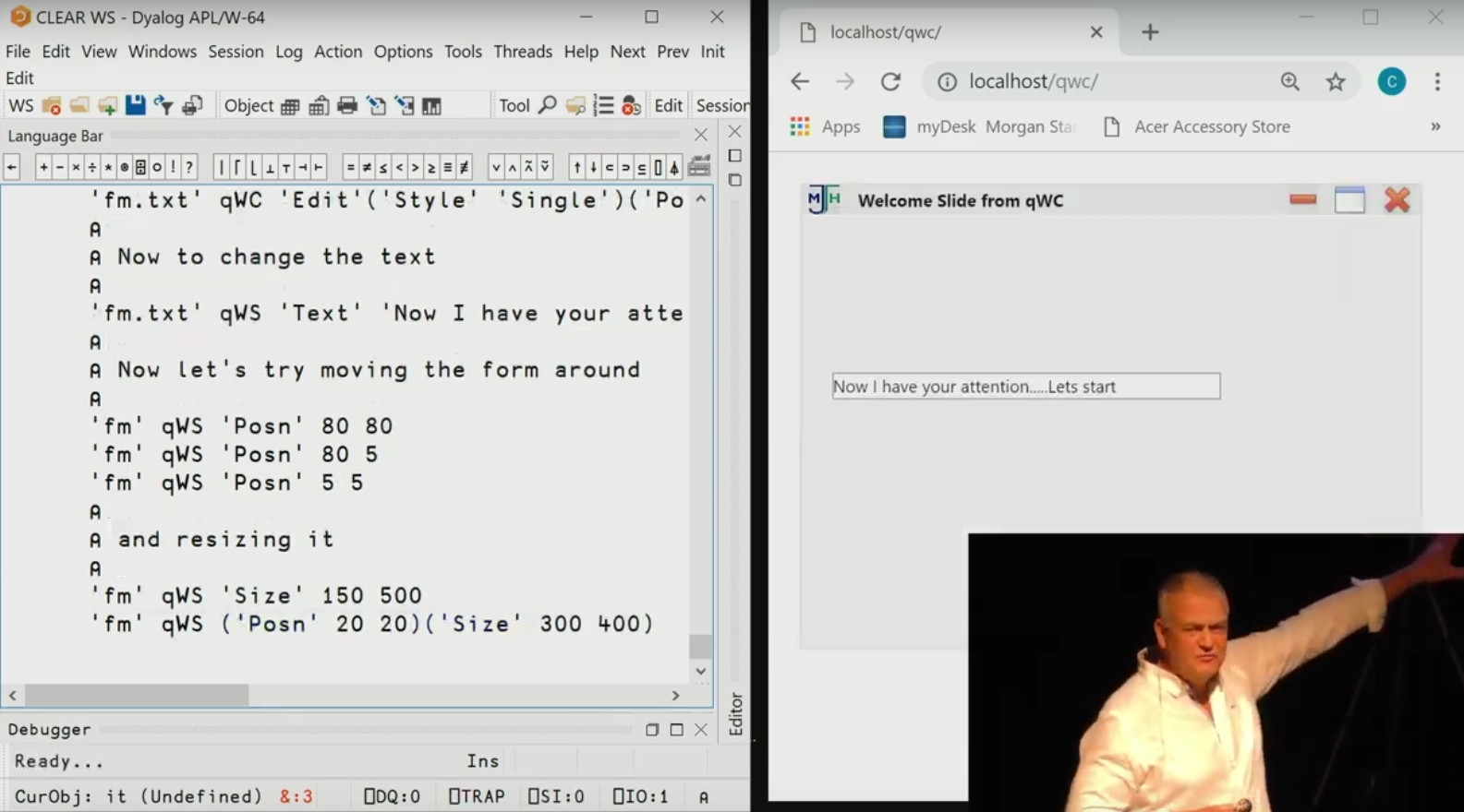
The upcoming release of version 17.1 includes a powerful new feature: the correctness–performance slider. To find this option, select Options>Configure>General in the IDE, or Edit>Preferences>General in RIDE. The slider is labelled “Execution Properties” and may be set at any time, although users should note that the effective correctness may be reduced if this is done while an in-progress function is on the stack.
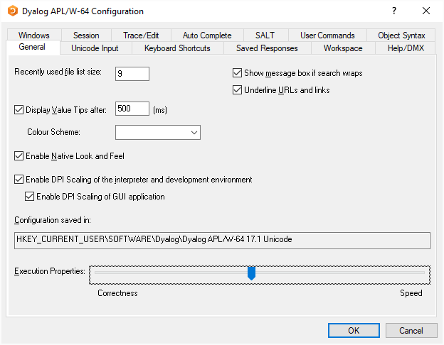
With the slider at its default position near the middle, Dyalog will make an effort to balance performance and correctness. Computations will proceed at a reasonably brisk pace, and slightly wrong answers will appear occasionally while very wrong ones come up only rarely. As the slider is moved to the left, correctness is increased at the expense of performance. You’ll have to wait for your results but when you get them they’ll be numbers you can trust. Moving the slider to the right will have the opposite effect, increasing speed at the expense of more frequent misparsings and significant floating point error. Perfect for startups!
Motivation
The seasoned programmer has most likely experienced the same issues as us, and may already be rushing to incorporate our ideas in his or her own code. In the interest of transparency, however, we wish to explain a bit further our experiences with the speed-correctness tradeoff.
Most often we encounter this tradeoff in one direction: when writing to improve the performance of a particular interpreter operation we sometimes find the results returned are different. In the past such cases were seen as bugs to be corrected, but we now understand them to simply be instances of a universal rule. Conversely, fixes for obscure parsing issues which slow down parsing of equally obscure but already correct cases are no longer cause for concern: we simply condition them on the appropriate slider threshold.
In the graph below we plot the accuracy and performance of several algorithms to compute the inner product !.○ on two large array arguments. Performance is measured in throughput (GB/s) while accuracy is defined to be the cosine similarity of the returned solution relative to a very precise result worked out with paper and pencil.
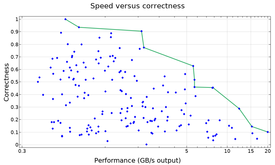
On plotting these results the nature of our plight became clear, and we added the performance-correctness slider to Dyalog version 17.1 as fast as possible. This post was written as accompaniment, with similar haste.
Results
We profiled a large sample program with many different execution settings and obtained the results shown below. As you can see, Dyalog can be quite stable, or quite fast, depending on how the performance-correctness slider is set.
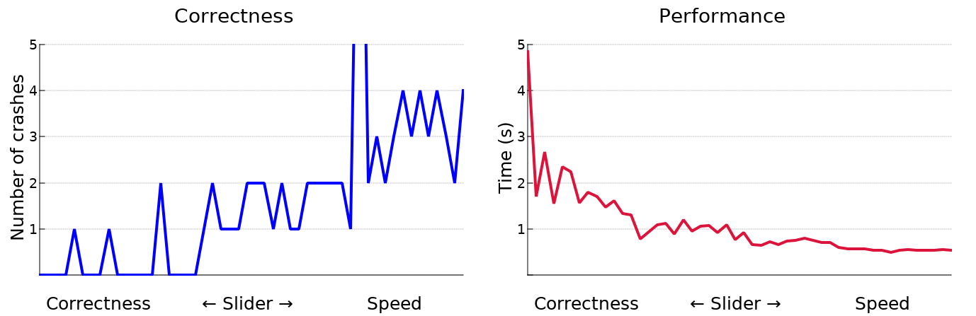
We believe these results demonstrate excellent value for all of our clients. Large and conscientious businesses can set the slider to correctness to encounter very few errors in execution. Rest assured, if errors are reported with these settings, we will do our best to shift them to the right side of the performance-correctness continuum! In contrast, the APL thrill-seeker will find much to like at the speedy end of the spectrum, as more frequent crashes are compounded by an interpreter that gets to them faster.
Future extensions
Although we believe the provided options will satisfy most users, some tasks require an implementation so fast, or so correct, that Dyalog cannot currently offer satisfactory performance along the relevant axis. To rectify this in the future we intend to offer more powerful facilities which extend the extremes of the correctness-performance slider. Potential clients who are exceptionally interested in correctness, such as NASA and Airbus, should contact us about an interpreter which runs multiple algorithms for each operation and chooses the majority result. For users interested in speed above all else we propose to offer an interpreter which only computes a part of its result and leaves the rest uninitialised, thus obtaining for example a 50% correct result in only half the time.
Even more extreme tradeoffs are possible. For the most correct results we are considering an algorithm which adds the desired computation to Wikipedia’s “List of unsolved problems in mathematics”, and then scans mathematical journals until a result with proof is obtained. For extremely fast responses we propose to train a shallow neural network on APL sessions so that it can, without interpreting any APL, print something that basically looks like it could be the right answer. Such an option would be a useful and efficient tool for programmers who cannot use APL, but insist on doing so anyway.
Although our plans for the future may be much grander, we’re quite excited to be the first language to offer user-selectable implementation tradeoffs at all. We’re sure you’ll be happy with either the correctness or the performance of Dyalog 17.1!
 Follow
 On June 30th 2018 she married Tom Fergus, Remy’s Dad, in a small ceremony at Trowbridge County Hall and became Jo Fergus. The wedding came as a bit of a surprise to friends and family who thought they were attending a birthday lunch but the sun shone and a fantastic day was had by all. Jo started to miss playing pool and in 2018 she went to the Wiltshire county pool trials and was invited back into the Wiltshire Ladies A county team. After a successful season, in which they didn’t lose a match, the team has qualified for National County Finals taking place at the beginning of March. Jo has also joined a team playing in her local pool league.