

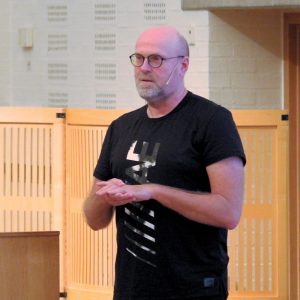
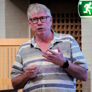
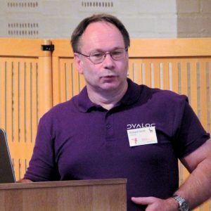
Claus Madsen of FinE Analytics
Scrinium is a portfolio management system that can handle a comprehensive range of financial assets, collect them into “portfolios”, and compute returns (SR, ANN, TWR), risk (Std, VaR, Duration, Convexit, Delta, Gamma, Sharpe) and relative risk (Alpha, Beta, Jensens Alpha, Tracking Error). It deals with benchmarks, and so on and so forth. However, Claus Madsen’s presentation at Dyalog ’19 doesn’t delve deeply into financial maths. Instead, his talk is mostly about the architecture of Scrinium. To allow himself to focus on all of the above-mentioned computations, Claus has organised all of his computations into classes, which he exposes as Microsoft.NET assemblies. This allows him to leave the production of user interfaces and other wrapping to “IT people”.
The other two presentations featured this week are about the statistical package TamStat. TamStat has a new graphical user interface based on the HTMLRenderer, which means that the interface is identical under Microsoft Windows, macOS and Linux.
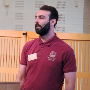
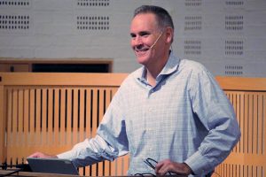
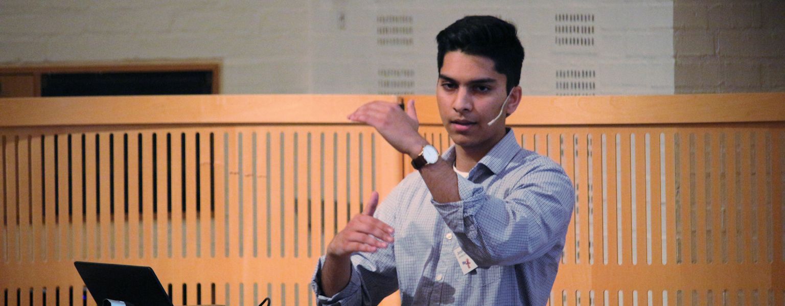
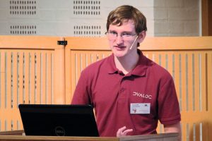
Richard Park talks TamStat
Stephen Mansour was unable to attend the Dyalog user meeting this year as he was busy teaching statistics using TamStat at Scranton University in Pennsylvania, US. In two talks at Dyalog ’19, Richard Park and Michael Baas provide two different perspectives on the new TamStat UI. First, Richard talks about the fundamental design of the underlying statistical language and how the UI guides inexperienced users and helps construct executable TamStat statements. Michael follows up with a talk on the implementation of the “Wizards” and other features of the new UI that he has worked on during 2019 in collaboration with Dr. Mansour.
Summary of this week’s videos:
 Follow
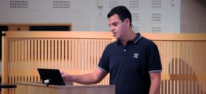

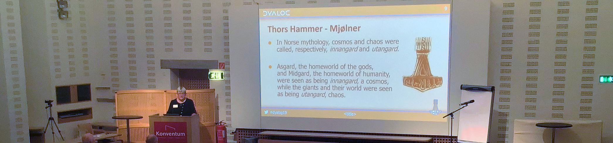
 2019 is the first “Year of the Hammer”: after seven years of Norse wyrms and seven years of Viking ships, we were now entering the era of seven hammer-inspired logos. As Gitte explains in her talk, we are celebrating the first year under Thor’s Hammer by making Dyalog APL freely available for non-commercial use – without requiring registration – under Microsoft Windows, Apple macOS and GNU/Linux (including a collection of public Docker images). The intention is to make APL much more easily accessible for experiments – especially in the cloud!
 After last year’s Technical Road Map, which was almost entirely a live demonstration of using APL with modern development tools like Git, VS Code and Docker, I decided to play it safe this year and do no demos at all in my keynote. Instead, I concentrated on explaining some of our thoughts about making Dyalog APL easier to discover, learn and integrate into modern frameworks and development processes – and making applications written in APL easier to deploy and maintain. As a result, despite the world premiere of our new Webinar Jingle, composed by Stefano Lanzavecchia (
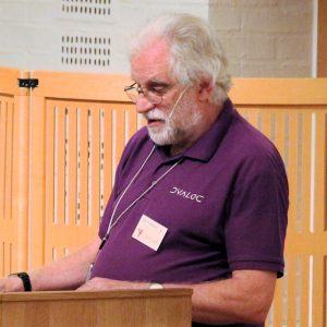
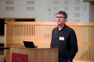
 The title of John’s talk was “Cor(e) Blimey!”. The Cor(e) is of course a reference to Microsoft’s “.NET Core” but if English is not your first language, the title of John’s talk may need a little explanation. “Cor blimey” is an exclamation of surprise, a euphemism derived from “God Blind Me”. In this talk, John explains how Dyalog is poised to provide a bridge to Microsoft’s new portable, open source version of .NET. Scheduled for release with Dyalog version 18.0 next year, this will provide APL users with access to a vast collection of libraries under Linux and macOS, in addition to Windows.