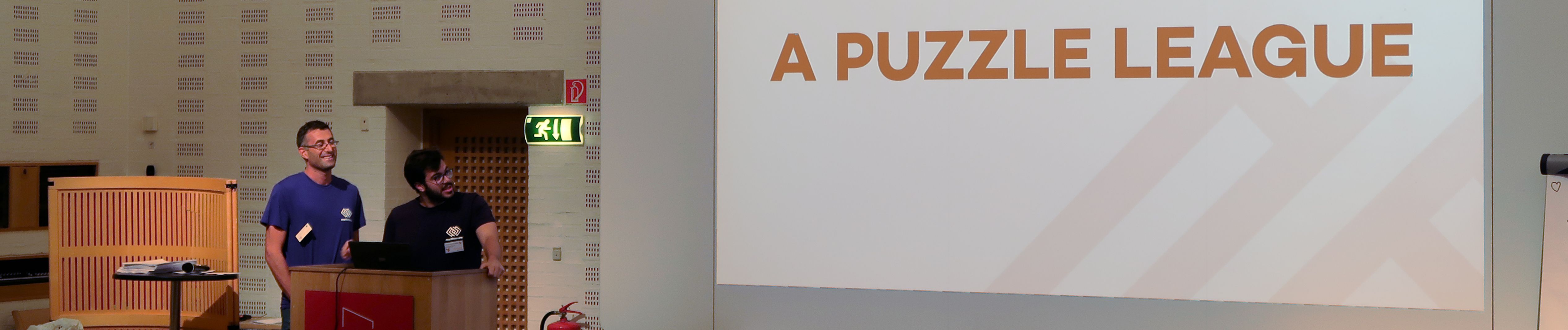

Dyalog Pictures Ltd?
After a wonderful banquet dinner bonding with fellow teammates of last night’s Viking Challenge, we were invited to the Jorns Auditorium for the world premiere of our movies from earlier in the day. The screening and awards show was a roaring success with everybody being surprised and thrilled at the quality of what came out from the editing room. We would like to thank Filmteambuilding.dk for an incredibly enjoyable afternoon and evening.
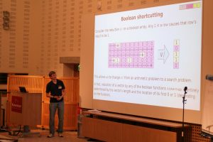
How do I… in APL?
In another world premiere, Adám Brudzewsky introduced us to APLcart this morning. This is the new answer to the question “how do I… in APL?”. Luckily Adám’s presentation strategy of asking the audience for functionality to search for was a win-win – if APLcart had it then we were impressed, and if not Adám had a new item to add to APLcart. Try it now and see if APLcart has what you’re looking for. If you can’t, Adám invites you to email the functions you want to see to adam(AT)aplcart.info.
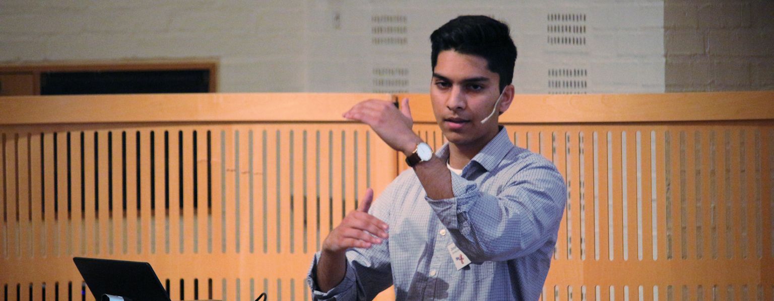
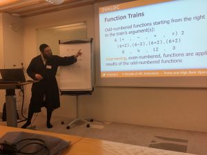
Richard Park then gave his third and final presentation of the week on the theme of using APL for education. He showed us how you can quickly and easily create Dyalog Jupyter notebooks and recommended using them for how-to, instructional documents and problem sets for students. You can view and download his presentation (which is a notebook) from GitHub, and interact with the live running notebook by clicking this button → ![]() .
.
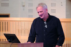
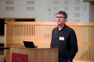
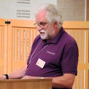
Tomas Gustafsson tells the Irma story
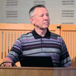
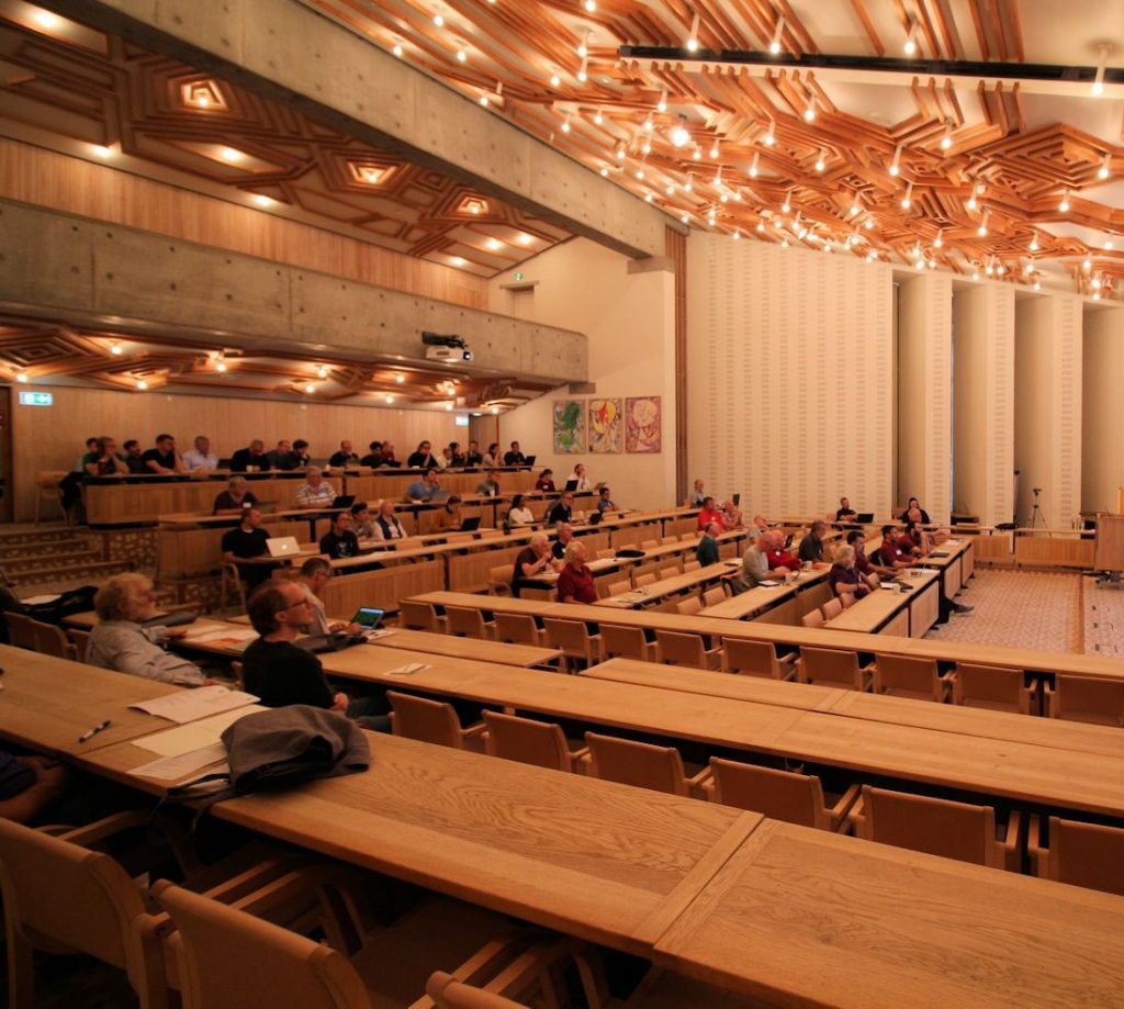
We then had the final talk of the User Meeting. Tomas Gustafsson, creator of the Stormwind boating simulator, told us the fascinating story of the Finnish ship M/S Irma. It disappeared while travelling a common route in 1968 and became one of the greatest mysteries in Finnish maritime history. Eventually some wreckage was found near Åland and Tomas was able to use APL, reconstructing possible paths of the debris via simulation, to make an educated guess of where to search for the main wreckage.
Lastly Gitte expressed to us how enjoyable the week had been, and all in the audience seemed to agree. We thanked Helene, Karen, Jason, Fiona and all of the staff at Konventum for their hard work “behind the scenes” to make the User Meeting run smoothly.
For the last afternoon of the User Meeting three final workshops were held. Two focused on technical software development issues, with Morten and Josh answering users’ questions related to using text-based source with ]LINK and Git. Andy Shiers and John Daintree were generally helping users with application-related issues, but were especially helpful to some of the young new users of APL. Some of our delegates took on another challenge in the workshop on code golfing.
I think it is safe to say that we have all thoroughly enjoyed this week. You can look forward to seeing our commercials from the Viking Challenge as well as recordings of talks from this week at some point in the future on dyalog.tv.
 Follow