Stencil Maneuvers

Introduction

The e-mail arrived in the early afternoon from Morten, in Finland attending the FinnAPL Forest Seminar.

How do I speed this up and impress the Finns?

0 cmpx 'e←⊃∨/0.2 edges¨r g b'
6.4E¯1
edges
{⍺←0.7 ⋄ 1 1↓¯1 ¯1↓⍺<(|EdgeDetect apply ⍵)÷1⌈(+⌿÷≢),⍵}
apply
{stencil←⍺ ⋄ {+/,⍵×stencil}⌺(⍴stencil)⊢⍵}
EdgeDetect
¯1 ¯1 ¯1
¯1 8 ¯1
¯1 ¯1 ¯1

(r g b in the attached ws)

Background

is stencil, a new dyadic operator which will be available in version 16.0. In brief, f⌺s applies the operand function f to windows of size s. The window is moved over the argument centered over every possible position. The size is commonly odd and the movement commonly 1. For example:

   {⊂⍵}⌺5 3⊢6 5⍴⍳30
┌───────┬────────┬────────┬────────┬───────┐
│0  0  0│ 0  0  0│ 0  0  0│ 0  0  0│ 0  0 0│
│0  0  0│ 0  0  0│ 0  0  0│ 0  0  0│ 0  0 0│
│0  1  2│ 1  2  3│ 2  3  4│ 3  4  5│ 4  5 0│
│0  6  7│ 6  7  8│ 7  8  9│ 8  9 10│ 9 10 0│
│0 11 12│11 12 13│12 13 14│13 14 15│14 15 0│
├───────┼────────┼────────┼────────┼───────┤
│0  0  0│ 0  0  0│ 0  0  0│ 0  0  0│ 0  0 0│
│0  1  2│ 1  2  3│ 2  3  4│ 3  4  5│ 4  5 0│
│0  6  7│ 6  7  8│ 7  8  9│ 8  9 10│ 9 10 0│
│0 11 12│11 12 13│12 13 14│13 14 15│14 15 0│
│0 16 17│16 17 18│17 18 19│18 19 20│19 20 0│
├───────┼────────┼────────┼────────┼───────┤
│0  1  2│ 1  2  3│ 2  3  4│ 3  4  5│ 4  5 0│
│0  6  7│ 6  7  8│ 7  8  9│ 8  9 10│ 9 10 0│
│0 11 12│11 12 13│12 13 14│13 14 15│14 15 0│
│0 16 17│16 17 18│17 18 19│18 19 20│19 20 0│
│0 21 22│21 22 23│22 23 24│23 24 25│24 25 0│
├───────┼────────┼────────┼────────┼───────┤
│0  6  7│ 6  7  8│ 7  8  9│ 8  9 10│ 9 10 0│
│0 11 12│11 12 13│12 13 14│13 14 15│14 15 0│
│0 16 17│16 17 18│17 18 19│18 19 20│19 20 0│
│0 21 22│21 22 23│22 23 24│23 24 25│24 25 0│
│0 26 27│26 27 28│27 28 29│28 29 30│29 30 0│
├───────┼────────┼────────┼────────┼───────┤
│0 11 12│11 12 13│12 13 14│13 14 15│14 15 0│
│0 16 17│16 17 18│17 18 19│18 19 20│19 20 0│
│0 21 22│21 22 23│22 23 24│23 24 25│24 25 0│
│0 26 27│26 27 28│27 28 29│28 29 30│29 30 0│
│0  0  0│ 0  0  0│ 0  0  0│ 0  0  0│ 0  0 0│
├───────┼────────┼────────┼────────┼───────┤
│0 16 17│16 17 18│17 18 19│18 19 20│19 20 0│
│0 21 22│21 22 23│22 23 24│23 24 25│24 25 0│
│0 26 27│26 27 28│27 28 29│28 29 30│29 30 0│
│0  0  0│ 0  0  0│ 0  0  0│ 0  0  0│ 0  0 0│
│0  0  0│ 0  0  0│ 0  0  0│ 0  0  0│ 0  0 0│
└───────┴────────┴────────┴────────┴───────┘
   {+/,⍵}⌺5 3⊢6 5⍴⍳30
 39  63  72  81  57
 72 114 126 138  96
115 180 195 210 145
165 255 270 285 195
152 234 246 258 176
129 198 207 216 147

In addition, for matrix right arguments with movement 1, special code is provided for the following operand functions:

{∧/,⍵}   {∨/,⍵}   {=/,⍵}   {≠/,⍵} 

{⍵}      {,⍵}     {⊂⍵}     {+/,⍵}

{+/,A×⍵}     {E<+/,A×⍵}       
{+/⍪A×⍤2⊢⍵}  {E<+/⍪A×⍤2⊢⍵}

The comparison < can be one of < ≤ = ≠ ≥ >.

The variables r g b in the problem are integer matrices with shape 227 316 having values between 0 and 255. For present purposes we can initialize them to random values:

   r←¯1+?227 316⍴256
   g←¯1+?227 316⍴256
   b←¯1+?227 316⍴256

Opening Moves

I had other obligations and did not attend to the problem until 7 PM. A low-hanging fruit was immediately apparent: {+/,⍵×A}⌺s is not implemented by special code but {+/,A×⍵}⌺s is. The difference in performance is significant:

   edges1←{⍺←0.7 ⋄ 1 1↓¯1 ¯1↓⍺<(|EdgeDetect apply1 ⍵)÷1⌈(+⌿÷≢),⍵}
   apply1←{stencil←⍺ ⋄ {+/,stencil×⍵}⌺(⍴stencil)⊢⍵}

   cmpx 'e←⊃∨/0.2 edges1¨r g b' 'e←⊃∨/0.2 edges ¨r g b'
  e←⊃∨/0.2 edges1¨r g b → 8.0E¯3 |     0% ⎕
  e←⊃∨/0.2 edges ¨r g b → 6.1E¯1 | +7559% ⎕⎕⎕⎕⎕⎕⎕⎕⎕⎕⎕⎕⎕⎕⎕⎕⎕⎕⎕⎕⎕⎕

I fired off an e-mail reporting this good result, then turned to other more urgent matters. An example of the good being an enemy of the better, I suppose.

When I returned to the problem at 11 PM, the smug good feelings have largely dissipated:

  • Why should {+/,A×⍵}⌺s be so much faster than {+/,⍵×A}⌺s? That is, why is there special code for the former but not the latter? (Answer: all the special codes end with … ⍵}.)
  • I can not win: If the factor is small, then why isn’t it larger; if it is large, it’s only because the original code wasn’t very good.
  • The large factor is because, for this problem, C (special code) is still so much faster than APL (magic function).
  • If the absolute value can somehow be replaced, the operand function can then be in the form {E<+/,A×⍵}⌺s, already implemented by special code. Alternatively, {E<|+/,A×⍵}⌺s can be implemented by new special code.

Regarding the last point, the performance improvement potentially can be:

   edges2←{⍺←0.7 ⋄ 1 1↓¯1 ¯1↓(⍺ EdgeDetect)apply2 ⍵}
   apply2←{threshold stencil←⍺ ⋄ 
                    {threshold<+/,stencil×⍵}⌺(⍴stencil)⊢⍵}

   cmpx (⊂'e←⊃∨/0.2 edges'),¨'21 ',¨⊂'¨r g b'
  e←⊃∨/0.2 edges2¨r g b → 4.8E¯3 |      0%
* e←⊃∨/0.2 edges1¨r g b → 7.5E¯3 |    +57%
* e←⊃∨/0.2 edges ¨r g b → 7.4E¯1 | +15489% ⎕⎕⎕⎕⎕⎕⎕⎕⎕⎕⎕⎕⎕⎕⎕⎕⎕⎕⎕⎕⎕

The * in the result of cmpx indicates that the expressions don’t give the same results. That is expected; edges2 is not meant to give the same results but is to get a sense of the performance difference. (Here, an additional factor of 1.57.)

edges1 has the expression ⍺<matrix÷1⌈(+⌿÷≢),⍵ where and the divisor are both scalars. Reordering the expression eliminates one matrix operation: (⍺×1⌈(+⌿÷≢),⍵)<matrix. Thus:

   edges1a←{⍺←0.7 ⋄ 1 1↓¯1 ¯1↓(⍺×1⌈(+⌿÷≢),⍵)<|EdgeDetect apply1 ⍵}

   cmpx (⊂'e←⊃∨/0.2 edges'),¨('1a' '1 ' '  '),¨⊂'¨r g b'
  e←⊃∨/0.2 edges1a¨r g b → 6.3E¯3 |      0%
  e←⊃∨/0.2 edges1 ¨r g b → 7.6E¯3 |    +22%
  e←⊃∨/0.2 edges  ¨r g b → 6.5E¯1 | +10232% ⎕⎕⎕⎕⎕⎕⎕⎕⎕⎕⎕⎕⎕⎕⎕⎕⎕⎕⎕⎕

The time was almost 1 AM. To bed.

Further Maneuvers

Fresh and promising ideas came with the morning. The following discussion applies to the operand function {+/,A×⍵}.

(0) Scalar multiple: If all the elements of A are equal, then {+/,A×⍵}⌺(⍴A)⊢r ←→ (⊃A)×{+/,⍵}⌺(⍴A)⊢r.

   A←3 3⍴?17
   ({+/,A×⍵}⌺(⍴A)⊢r) ≡ (⊃A)×{+/,⍵}⌺(⍴A)⊢r
1

(1) Sum v inner product: {+/,⍵}⌺(⍴A)⊢r is significantly faster than {+/,A×⍵}⌺(⍴A)⊢r because the former exploits mathematical properties absent from the latter.

   A←?3 3⍴17
   cmpx '{+/,⍵}⌺(⍴A)⊢r' '{+/,A×⍵}⌺(⍴A)⊢r'
  {+/,⍵}⌺(⍴A)⊢r   → 1.4E¯4 |    0% ⎕⎕⎕
* {+/,A×⍵}⌺(⍴A)⊢r → 1.3E¯3 | +828% ⎕⎕⎕⎕⎕⎕⎕⎕⎕⎕⎕⎕⎕⎕⎕⎕⎕⎕⎕⎕⎕⎕⎕⎕⎕⎕⎕⎕⎕

(The * in the result of cmpx is expected.)

(2) Linearity: the stencil of the sum equals the sum of the stencils.

   A←?3 3⍴17
   B←?3 3⍴17
   ({+/,(A+B)×⍵}⌺(⍴A)⊢r) ≡ ({+/,A×⍵}⌺(⍴A)⊢r) + {+/,B×⍵}⌺(⍴A)⊢r 
1

(3) Middle: If B is zero everywhere except the middle, then {+/,B×⍵}⌺(⍴B)⊢r ←→ mid×r where mid is the middle value.

   B←(⍴A)⍴0 0 0 0 9
   B
0 0 0
0 9 0
0 0 0
   ({+/,B×⍵}⌺(⍴B)⊢r) ≡ 9×r
1

(4) A faster solution.

   A←EdgeDetect
   B←(⍴A)⍴0 0 0 0 9
   C←(⍴A)⍴¯1
   A B C
┌────────┬─────┬────────┐
│¯1 ¯1 ¯1│0 0 0│¯1 ¯1 ¯1│
│¯1  8 ¯1│0 9 0│¯1 ¯1 ¯1│
│¯1 ¯1 ¯1│0 0 0│¯1 ¯1 ¯1│
└────────┴─────┴────────┘
   A ≡ B+C
1

Whence:

   ({+/,A×⍵}⌺(⍴A)⊢r) ≡ ({+/,B×⍵}⌺(⍴A)⊢r) + {+/,C×⍵}⌺(⍴A)⊢r ⍝ (2)
1
   ({+/,A×⍵}⌺(⍴A)⊢r) ≡ ({+/,B×⍵}⌺(⍴A)⊢r) - {+/,⍵}⌺(⍴A)⊢r   ⍝ (0)
1
   ({+/,A×⍵}⌺(⍴A)⊢r) ≡ (9×r) - {+/,⍵}⌺(⍴A)⊢r                ⍝ (3)
1

Putting it all together:

edges3←{
  ⍺←0.7
  mid←⊃EdgeDetect↓⍨⌊2÷⍨⍴EdgeDetect
  1 1↓¯1 ¯1↓(⍺×1⌈(+⌿÷≢),⍵)<|(⍵×1+mid)-{+/,⍵}⌺(⍴EdgeDetect)⊢⍵
}

Comparing the various edges:

   x←(⊂'e←⊃∨/0.2 edges'),¨('3 ' '2 ' '1a' '1 ' '  '),¨⊂'¨r g b'
   cmpx x
  e←⊃∨/0.2 edges3 ¨r g b → 3.4E¯3 |      0%
* e←⊃∨/0.2 edges2 ¨r g b → 4.3E¯3 |    +25%
  e←⊃∨/0.2 edges1a¨r g b → 6.4E¯3 |    +88%
  e←⊃∨/0.2 edges1 ¨r g b → 7.5E¯3 |   +122%
  e←⊃∨/0.2 edges  ¨r g b → 6.5E¯1 | +19022% ⎕⎕⎕⎕⎕⎕⎕⎕⎕⎕⎕⎕⎕⎕⎕⎕⎕⎕⎕⎕
edges original
edges1 uses {+/,stencil×⍵} instead of {+/,⍵×stencil}
edges1a uses (⍺×mean,⍵)<matrix instead of ⍺<matrix÷mean,⍵
edges2 uses {threshold<+/,stencil×⍵}
edges3 uses the faster {+/,⍵} instead of {+/,stencil×⍵} and other maneuvers

Fin

I don’t know if the Finns would be impressed. The exercise has been amusing in any case.

Displaying cross-references with SharpPlot

Requirements: Update SharpPlot to v3.37 from my.dyalog.com > Downloads > Tools & Interfaces > GUI Tools > SharpPlot

SharpPlot v3.37 introduces Network Maps as a new chart type, and we’re going to use it to display the output of the ]XRef user command, which displays cross-references between all kinds of APL names :

      ]XRef ⎕SE.Parser
             DDEEEFLLMMNNPPPPPPPPPPPQQSSSTUaaaabbbcdddddddfffiilmmmmmmnnnnnnppppqqqqrrrsssssssssstttttuvvvxx∆⍵⍺ 
             EeRnrOOSAOAsRrsssssssss.uwwwrPrrrr:alu.aaaeee.ei.fq.aeioo.adeop.Daa.1mq.et:eipqtwwww:aqwxp.an.C... 
             LlRd:RW.XDRwEo:.eeeeeee.oDTiaPgggg:d.t.tttQff.ax.:..smndd..awv..art..:..qb:t.lzr.imp:b.vtp.lc.u... 
             I.OT:CE.APGiFp:Pttttttt.t.atpE.psv:....aaau.i.tC.:..k.lei..:....tm...:....:..i.:.tao:l...e....t... 
             M.Rr:ER.ROStIa:a........e.bc.R.o.a:....:..o.n.ua.:....elf..:....as...:....:..t.:..ts:e...r....:... 
             I.0a:S..GS.cXg:r.Samnpu.s.lh.:.s.l:....:ASt.e.rs.:....n.i..:....:....:....:..P.:....:....C....:... 
             T..p:P..S:.h.a:s.wloarp.:.e..:...u:....:rwe.d.ee.:....:.e..:....:....:....:..a.:....:....a....:... 
             E...:A...:.e.t:e.ildrep.:....:...e:....:gD..:.s..:....:.r..:....:....:....:..r.:....:....s....:... 
             R...:C...:.s.e:..toigfe.:....:...s:....:u...:....:....:.s..:....:....:....:..m.:....:....e....:... 
             ....:E...:....:..cwfsir.:....:....:....:m...:....:....:....:....:....:....:..s.:....:....:....:... 
             ....:....:....:..hni.x..:....:....:....:e...:....:....:....:....:....:....:....:....:....:....:... 
             ....:....:....:...oe....:....:....:....:n...:....:....:....:....:....:....:....:....:....:....:... 
             ....:....:....:...sr....:....:....:....:t...:....:....:....:....:....:....:....:....:....:....:... 
             ....:....:....:...ps....:....:....:....:s...:....:....:....:....:....:....:....:....:....:....:... 
             ....:....:....:...a:....:....:....:....:....:....:....:....:....:....:....:....:....:....:....:... 
             ....:....:....:...c:....:....:....:....:....:....:....:....:....:....:....:....:....:....:....:... 
             ....:....:....:...e:....:....:....:....:....:....:....:....:....:....:....:....:....:....:....:... 
 [FNS]        - - - - : - - - - : - - - - : - - - - : - - - - : - - - - : - - - - : - - - - : - - - - : - - - - 
 Parse       G.GG○G G GGGG. . . : . ○F.G.G:○○○○○! . ○GGF.○. .○F ○ .○. . ○!○○○G○○! : .○○○○ F :○○○○○○ ○ : ○○.F! . 
 Propagate    ○ . . . : . . . . : . . G . : . .○. . : . . . . : . . .○. : . . . . : . . .○. ○○. . . . :○. . . . 
 Quotes       . . . . : . . . . : . ○ . . : . . . . : . . . .○: .○. . ○ : . . . . ○ . . . . ○ . . .○. : . . . . 
 Switch       . G . . : . . . . : . . G .G: . . . . : . ○ . . : . . . . : . . . . : ○ .○. . : . . . . :○. . . . 
 deQuote      . . . . : . . . . : . . . . : . . . . : . . . . :○○ . . . : . . . . : . . . . ○ . . . . : . . . . 
 fixCase      . . . . : . . . . : . . . . : . . . . : . . . . : . . . . : . . . . : . . . . : . . . . : . . .○. 
 if           . . . . : . . . . : . . . . : . . . . : . . . . : . . . . : . . . . : . . . . : . . . . : . . . . 
 init        G.G. G GGGGGGFGGGGGGGGG.F.GF :○. .○. ○ : . . ○○F F . ○ ○ ○○: . .G. . : . . . .F: . . . . F . GF. . 
 splitParms   . . . . : . . . . : . ○ . . : . . .○.○: . . . . : . . . ○ : .○○ ○ ○○:○. .○. . : . .○. .○: . . . . 
 sqz          . . . . : . . . . : . . . . : . .○. . : . . . . : . . . . : . . . . : . .○. . : . . . . : . . .○. 
 upperCase    . . .G. : . . . . : . . . . G . .○. . : . . . .○: . . . . : . . . . : . .○. . : . . . . : . . .○. 
 xCut         . . . . : . . . . : . . . . : . . . . : . . . . : . . . . : . . . . : . . . . : . . . . : . . .○○ 

We can capture the output of the user command by doing either
]mat←XRef ⎕SE.Parser (from session)
or
mat←⎕SE.UCMD']XRef ⎕SE.Parser' (from code)

Until Dyalog v16.0 (which has ]XRef -raw), we need to parse the output of ]XRef to get a square link matrix, along with the full list of nodes (in row/column order of the matrix) and list of original rows (functions).

    ∇ (mat nodes rows)←GetMatrix mat;nodelabs;rows;cols;labs;cat;diag
      (rows mat)←2↑(1,2</∧⌿mat=' ')⊂[2]mat        ⍝ cut at empty column
      (cols mat)←2↑(1,2<⌿∧/mat∊' -:')⊂[1]mat      ⍝ cut at - - - - : - - - -
      mat←1↓[1](' '∨.≠mat)/mat                    ⍝ trim first row and empty columns
      rows←~∘' '¨↓(-1⊃⍴mat)↑[1]rows               ⍝ row titles (list of strings)
      cols←~∘' .:'¨↓(-2⊃⍴mat)↑[1]⍉cols            ⍝ col titles (list of strings)
      nodes←rows∪cols                             ⍝ all titles
      mat←((mat,' ')⍪' ')[rows⍳nodes;cols⍳nodes]  ⍝ square matrix of nodes
    ∇

Now let’s wrap the SharpPlot initialisation into a single function that uses the .NET version if available and falls back to the cross-platform APL workspace if not:

    ∇ {dotnet}←Init
      :If dotnet←(,'W')≡3⊃'.'⎕WG'APLVersion'
          ⍝ .Net assembly (windows only)
          ⎕USING←',sharpplot.dll' ',system.drawing.dll'
      :Else
          ⍝ APL workspace (all platforms)
          :If 0=⎕NC'Causeway'   ⍝ copy workspace only once
              (System.Drawing←System←⍎'Causeway'⎕NS'').(⎕CY'sharpplot.dws')
          :EndIf 
      :EndIf
    ∇

Then we can write a platform-independent function that returns the SharpPlot instance with the chart drawn on it. We split nodes into two categories, functions and globals (ignoring locals and labels) and split links by destination node. By default, DrawNetworkMap lays out node categories on co-centric circles. Also, because the graph is uni-directional, we can afford to use straight links without damaging readability:

    ∇ sp←name Plot(mat nodes rows);catlabs;nodecat
      sp←⎕NEW Causeway.SharpPlot
     
      catlabs←'Function' 'Global'    ⍝ links are split by destination node
      nodecat←(≢nodes)⍴0             ⍝ ignored by default
      ((∨⌿mat∊'FR*')/nodecat)←1      ⍝ functions
      ((∨⌿mat∊'G')/nodecat)←2        ⍝ globals
      ((nodes∊rows)/nodecat)←1       ⍝ caller functions
     
      sp.Heading←name
      sp.HeadingStyle←Causeway.HeadingStyles.Left
      sp.SetMargins 40 30 30 30
      sp.KeyStyle←Causeway.KeyStyles.(BottomAlign+RightAlign)
      sp.SetILabels⊂nodes
      sp.SetILabelFont'Arial' 6 System.Drawing.FontStyle.Bold System.Drawing.Color.Black
      sp.SetColors⊂System.Drawing.Color.(SkyBlue LightCoral)
      sp.SetMarkers Causeway.Marker.Ball
      sp.SetMarkerScales 2
      sp.SetLineStyles Causeway.LineStyle.Solid
      sp.SetPenWidths 0.5
      sp.NetworkMapStyle←Causeway.NetworkMapStyles.(SplitByDestination+Dissected+ArrowLines+FixedArcs+NoAxes+NoLinkKey)
      sp.SetNetworkMapLinkArc 0         ⍝ straight lines
      sp.SetArrowStyle 5                ⍝ fixed-size arrows
     
      sp.SplitBy nodecat catlabs
      sp.DrawNetworkMap⊂↓(mat∊'GFR*')   ⍝ use a single width for all valid links
    ∇

We can then save the graph as SVG to a file (here we use the SvgMode that scales the SVG to fit its container):
sp.SaveSvg 'XRef.svg' Causeway.SvgMode.FixedAspect

Or, if feeding a web server or renderer, we can grab the SVG as a single string without writing to disk:
svg←sp.RenderSvg Causeway.SvgMode.FixedAspect

Windows users will be able to use the SharpPlot Viewer:
vw←⎕NEW Causeway.SharpPlotViewer sp
vw.Show ⍬

XRef

More examples of Network Maps can be found on the SharpPlot.com website in the Network Map Tutorials. To translate C# examples into APL, you can refer to the SharpPlot Rosetta Stone.

Calculation v Look-Up

(⎕io←0 and timings are done in Dyalog version 15.0.)

Table Look-Up

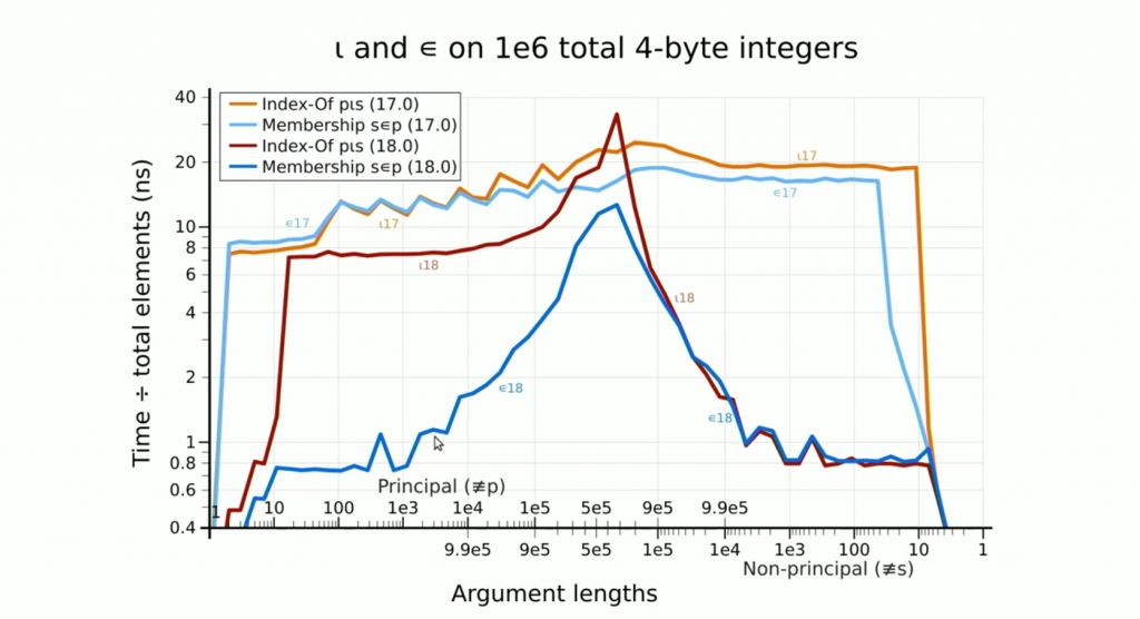
Some functions can be computed faster by table look-up than a more traditional and more conventional calculation. For example:

      b←?1e6⍴2

      cmpx '*b' '(*0 1)[b]'
 *b        → 1.32E¯2 |   0% ⎕⎕⎕⎕⎕⎕⎕⎕⎕⎕⎕⎕⎕⎕⎕⎕⎕⎕⎕⎕⎕⎕⎕⎕⎕⎕⎕⎕⎕⎕
 (*0 1)[b] → 1.23E¯3 | -91% ⎕⎕⎕

Some observations about this benchmark:

(a) The advantage of table look-up depends on the time to calculate the function directly, versus the time to do indexing, ⍺[⍵] or ⍵⌷⍺, plus a small amount of time to calculate the function on a (much) smaller representative set.

Indexing is particularly efficient when the indices are boolean:

      bb←b,1
      bi←b,2
      cmpx '2 3[bb]' '2 3 3[bi]'
 2 3[bb]   → 1.12E¯4 |    0% ⎕⎕⎕⎕⎕
 2 3 3[bi] → 7.39E¯4 | +558% ⎕⎕⎕⎕⎕⎕⎕⎕⎕⎕⎕⎕⎕⎕⎕⎕⎕⎕⎕⎕⎕⎕⎕⎕⎕⎕⎕⎕⎕⎕

bi is the same as bb except that the last element of 2 forces it to be 1-byte integers (for bi) instead of 1-bit booleans (for bb).

(b) Although the faster expression works best with 0-origin, the timing for 1-origin is similar.

      cmpx '*b' '{⎕io←0 ⋄ (*0 1)[⍵]}b'
 *b                   → 1.32E¯2 |   0% ⎕⎕⎕⎕⎕⎕⎕⎕⎕⎕⎕⎕⎕⎕⎕⎕⎕⎕⎕⎕⎕⎕⎕⎕⎕⎕⎕⎕⎕⎕
 {⎕io←0 ⋄ (*0 1)[⍵]}b → 1.22E¯3 | -91% ⎕⎕⎕

That is, if the current value of ⎕io is 1, the implementation can use a local ⎕io setting of 0.

(c) The fact that *b is currently slower than (*0 1)[b] represents a judgment by the implementers that *b is not a sufficiently common computation to warrant writing faster code for it. Other similar functions already embody the table look-up technique:

      cmpx '⍕b' '¯1↓,(2 2⍴''0 1 '')[b;]'
 ⍕b                   → 6.95E¯4 |  0% ⎕⎕⎕⎕⎕⎕⎕⎕⎕⎕⎕⎕⎕⎕⎕⎕⎕⎕⎕⎕⎕⎕⎕⎕⎕⎕⎕⎕⎕⎕
 ¯1↓,(2 2⍴'0 1 ')[b;] → 6.92E¯4 | -1% ⎕⎕⎕⎕⎕⎕⎕⎕⎕⎕⎕⎕⎕⎕⎕⎕⎕⎕⎕⎕⎕⎕⎕⎕⎕⎕⎕⎕⎕⎕

Small Domains

Table look-up works best for booleans, but it also works for other small domains such as 1-byte integers:

      i1←?1e6⍴128    ⍝ 1-byte integers

      cmpx '*i1' '(*⍳128)[i1]'
 *i1         → 1.48E¯2 |   0% ⎕⎕⎕⎕⎕⎕⎕⎕⎕⎕⎕⎕⎕⎕⎕⎕⎕⎕⎕⎕⎕⎕⎕⎕⎕⎕⎕⎕⎕⎕
 (*⍳128)[i1] → 9.30E¯4 | -94% ⎕⎕

      cmpx '○i1' '(○⍳128)[i1]'
 ○i1         → 2.78E¯3 |   0% ⎕⎕⎕⎕⎕⎕⎕⎕⎕⎕⎕⎕⎕⎕⎕⎕⎕⎕⎕⎕⎕⎕⎕⎕⎕⎕⎕⎕⎕⎕
 (○⍳128)[i1] → 9.25E¯4 | -67% ⎕⎕⎕⎕⎕⎕⎕⎕⎕⎕

In general, a table for 1-byte integers needs to have values for ¯128+⍳256. Here ⍳128 is used to simulate that in C indexing can be done on 1-byte indices without extra computation on the indices. In APL, general 1-byte indices are used as table[i1+128]; in C, the expression is (table+offset)[i].

Domains considered “small” get bigger all the time as machines come equipped with ever larger memories.

Larger Domains

Table look-up is applicable when the argument is not a substantial subset of a large domain and there is a fast way to detect that it is not.

      i4s←1e7+?1e6⍴1e5    ⍝ small-range 4-byte integers

      G←{(⊂u⍳⍵)⌷⍺⍺ u←∪⍵}

      cmpx '⍟i4s' '⍟G i4s'
 ⍟i4s   → 1.44E¯2 |   0% ⎕⎕⎕⎕⎕⎕⎕⎕⎕⎕⎕⎕⎕⎕⎕⎕⎕⎕⎕⎕⎕⎕⎕⎕⎕⎕⎕⎕⎕⎕
 ⍟G i4s → 9.59E¯3 | -34% ⎕⎕⎕⎕⎕⎕⎕⎕⎕⎕⎕⎕⎕⎕⎕⎕⎕⎕⎕⎕

The definition of G implements that the argument is not used directly as indices (as in (⊂⍵)⌷⍺⍺ u) but needed to be looked up, the u⍳⍵ in (⊂u⍳⍵)⌷⍺⍺ u. Thus both index-of and indexing are key enablers for making table look-up competitive.

§4.3 of Notation as a Tool of Thought presents a different way to distribute the results of a calculation on the “nub” (unique items). But it takes more time and space and is limited to numeric scalar results.

      H←{(⍺⍺ u)+.×(u←∪⍵)∘.=⍵}

      i4a←1e7+?1e4⍴1e3    ⍝ small-range 4-byte integers

      cmpx '⍟i4a' '⍟G i4a' '⍟H i4a'
 ⍟i4a   → 1.56E¯4 |       0%
 ⍟G i4a → 6.25E¯5 |     -60%
 ⍟H i4a → 1.78E¯1 | +113500% ⎕⎕⎕⎕⎕⎕⎕⎕⎕⎕⎕⎕⎕⎕⎕⎕⎕⎕⎕⎕⎕⎕⎕⎕⎕⎕⎕⎕⎕⎕

The benchmark is done on the smaller i4a as a benchmark on i4s founders on the ≢∪⍵ by ≢⍵ boolean matrix (for i4s, 12.5 GB = ×/ 0.125 1e5 1e6) created by H.

Mathematical Background

New Math” teaches that a function is a set of ordered pairs whose first items are unique:

*⍵: {(⍵,*⍵)|⍵∊C}      The set of all (⍵,*⍵) where is a complex number
⍟⍵: {(⍵,⍟⍵)|⍵∊C~{0}}  The set of all (⍵,⍟⍵) where is a non-zero complex number
○⍵: {(⍵,○⍵)|⍵∊C}      The set of all (⍵,○⍵) where is a complex number
⍕⍵: {(⍵,⍕⍵)|0=⍴⍴⍵}    The set of all (⍵,⍕⍵) where is a scalar

When is restricted (for example) to the boolean domain, the functions, the sets of ordered pairs, are more simply represented by enumerating all the possibilities:

*⍵: {(0,1), (1,2.71828)}
⍟⍵: {(0,Err), (1,0)}
○⍵: {(0,0), (1,3.14159)}
⍕⍵: {(0,'0'), (1,'1')}

Realized and Potential Performance Improvements

realized (available no later than 15.0)

boolean
1-byte integer
⍕ ∘.f
⍕     a∘⍕

potential (non-exhaustive list)

boolean
1-byte integer
2-byte integer
small-range 4-byte integer
* ⍟ | - ○   ! ⍳ a∘f f.g
* ⍟ | - ○ × ! ⍳ a∘f f.g ∘.f
* ⍟ | - ○ ×   ⍳ a∘f
* ⍟ |     ×

a is a scalar; f and g are primitive scalar dyadic functions.

Supporting the Community – Update

You may have been wondering what has been happening with Jo Shaw (daughter of our Customer Account Manager, Karen) the England pool player who Dyalog have sponsored in the past, so we thought it was time for an update.

After getting a new job in December 2014, Jo moved from Hampshire to Wiltshire and joined the Wiltshire Ladies county pool team. After a successful first season with them, Jo again qualified to play for England as a reserve player in May 2016 but the exciting news that she was expecting a baby meant that she was not able to take up her place in the team – unfortunately the Nation’s Cup event was happening at the exact same time the baby was due. Jo also found that she was not able to practice or play pool during the later stages of her pregnancy as she was just not able to bend over the table(!) so this meant she had to take a back seat with the Wiltshire Ladies county team too.

Jo’s daughter Remy was born on 18 October 2016 and Remy has been a keen supporter of Wiltshire Ladies since she was born – she even has her own team shirt!

Jo and Remy have recently been to the EBPF National Finals to support Jo’s Wiltshire teammates as they became National Ladies Champions for the first time. Jo was disappointed that she wasn’t able to play a bigger part in the victory but being a mother is now her top priority and she was pleased that her team did so well.

After a lot of thought Jo has now made the very difficult decision to take some time out from both county and national pool to concentrate on being a mum. She plans to be back in a year or so once Remy is a bit older and Dyalog fully expect her to win back her place in the England team – we will be there to support her when she does!

Beauty and the Beast

beauty-and-the-beastFinally, the last accessory I ordered for my Raspberry Pi Zero (that’s the little red thing behind my keyboard) has arrived – an Acer 43″ ET430K monitor. The Zero won’t quite drive this monitor at its maximum resolution of 3840×2160 pixels, but as you can see, you get enough real estate to do real graphics with “ASCII Art” (well, Unicode Art, anyway)!

Some readers will recognise the image as the famous Mandelbrot Set, named after the mathematician Benoit Mandelbrot, who studied fractals. According to Wikipedia a fractal is a mathematical set that exhibits a repeating pattern displayed at every scale – they are interesting because they produce patterns that are very similar to things we can see around us – both in living organisms and landscapes – they seem to be part of the fundamental fabric of the universe.

Fractals are are also interesting because they produce images of staggering beauty, as you can see on the pages linked to above and one of our rotating banner pages, where a one-line form of the APL expression which produced the image is embedded:

Website_banner_MbrotW

The colourful images of the Mandelbrot set are produced by looking at a selection of points in the complex plane. For each point c, start with a value of 0 for z, repeat the computation z = c + z², and colour the point according to the number of iterations required before the function becomes “unbounded in value”.

In APL, the function for each iteration can be expressed as {c+⍵*2}, where c is the point and ⍵ (the right argument of the function) is z (initially 0, and subsequently the result of the previous iteration):

      f←{c+⍵*2} ⍝ define the function
      c←1J1     ⍝ c is 1+i (above and to the right of the set)
      (f 0)(f f 0)(f f f 0)(f f f f 0) (f f f f f 0)
1J1 1J3 ¯7J7 1J¯97 ¯9407J¯193

If you are not familiar with complex numbers, those results may look a bit odd. While complex addition just requires adding the real and the imaginary parts independently, the result of multiplication of two complex numbers (a + bi) and (c + di) is defined as (ac-db) + (bc+ad)i. Geometrically, complex multiplication is a combined stretching and rotation operation.

Typing all those f’s gets a bit tedious, fortunately APL has a power operator , a second-order function that can be used to repeatedly apply a function. We can also compute the magnitude of the result number using |:

      (|(f⍣6)0)(|(f⍣7)0)
8.853E7 7.837E15

Let’s take a look at what happens if we choose a point inside the Mandelbrot set:

      c←0.1J0.1
      {|(f⍣⍵)0}¨ 1 2 3 4 5 6 7 8 9 10
0.1414 0.1562 0.1566 0.1552 0.1547 0.1546 0.1546 0.1546 0.1546 0.1546

Above, I used an anonymous function so I could pass the number of iterations in as a parameter, and use the each operator ¨ to generate all the results up to ten iterations. In this case, we can see that the magnitude of the result stabilises, which is why the point 0.1 + 0.1i is considered to be inside the Mandelbrot set.

Points which are just outside the set will require varying numbers of applications of f before the magnitude “explodes”, and if you colour points according to how many iterations are needed and pick interesting areas along the edge of the set, great beauty is revealed.

1200px-GalaxyOfGalaxies

The above image is in the public domain and was created by Jonathan J. Dickau using ChaosPro 3.3 software, which was created by Martin Pfingstl.

Our next task is to create array of points in the complex plane. A helper function unitstep generates values between zero and 1 with a desired number of steps, so I can vary the resolution and size of the image. Using it, I can create two ranges, multiply one of them by i (0J1 in APL) and use an addition table (∘.+) to generate the array:

      ⎕io←0 ⍝ use index origin zero
      unitstep←{(⍳⍵+1)÷⍵}
      unitstep 6
0 0.1667 0.3333 0.5 0.6667 0.8333 1
      c←¯3 × 0.7J0.5 - (0J1×unitstep 6)∘.+unitstep 6
      c
¯2.1J¯1.5 ¯1.6J¯1.5 ¯1.1J¯1.5 ¯0.6J¯1.5 ¯0.1J¯1.5 0.4J¯1.5 0.9J¯1.5
¯2.1J¯1   ¯1.6J¯1   ¯1.1J¯1   ¯0.6J¯1   ¯0.1J¯1   0.4J¯1   0.9J¯1  
¯2.1J¯0.5 ¯1.6J¯0.5 ¯1.1J¯0.5 ¯0.6J¯0.5 ¯0.1J¯0.5 0.4J¯0.5 0.9J¯0.5
¯2.1      ¯1.6      ¯1.1      ¯0.6      ¯0.1      0.4      0.9     
¯2.1J00.5 ¯1.6J00.5 ¯1.1J00.5 ¯0.6J00.5 ¯0.1J00.5 0.4J00.5 0.9J00.5
¯2.1J01   ¯1.6J01   ¯1.1J01   ¯0.6J01   ¯0.1J01   0.4J01   0.9J01  
¯2.1J01.5 ¯1.6J01.5 ¯1.1J01.5 ¯0.6J01.5 ¯0.1J01.5 0.4J01.5 0.9J01.5

The result is subtracted from 0.7J0.5 (0.7 + 0.5i) to get the origin of the complex plane slightly off centre in the middle, and multiplied the whole thing by 3 to get a set of values that brackets the Mandelbrot set.

Note that APL expressions are typically rank and shape invariant, so our function f can be applied to the entire array without changes. Since our goal is only to produce ASCII art, we don’t need to count iterations, we can just compare the magnitude of the result with 9 to decide whether the point has escaped:

      9<|f 0
0 0 0 0 0 0 0
0 0 0 0 0 0 0
0 0 0 0 0 0 0
0 0 0 0 0 0 0
0 0 0 0 0 0 0
0 0 0 0 0 0 0
0 0 0 0 0 0 0
      9<|(f⍣3) 0 ⍝ Apply f 3 times
1 1 1 0 0 0 1
1 0 0 0 0 0 0
0 0 0 0 0 0 0
0 0 0 0 0 0 0
0 0 0 0 0 0 0
1 0 0 0 0 0 0
1 1 1 0 0 0 1

We can see that points around the edge start escaping after 3 iterations. Using an anonymous function again, we can observe more and more points escape, until we recognise the (very low resolution) outline of the Mandelbrot set:


      ]box on
      {((⍕⍵)@(⊂0 0))' #'[9>|(f⍣⍵)0]}¨2↓⍳9
┌───────┬───────┬───────┬───────┬───────┬───────┬───────┐
│2######│3  ### │4      │5      │6      │7      │8      │
│#######│ ######│   ### │    #  │    #  │    #  │    #  │
│#######│#######│ ##### │  #### │  #### │   ### │   ### │
│#######│#######│###### │ ##### │ ##### │ ##### │ ####  │
│#######│#######│ ##### │  #### │  #### │   ### │   ### │
│#######│ ######│   ### │    #  │    #  │    #  │    #  │
│#######│   ### │       │       │       │       │       │
└───────┴───────┴───────┴───────┴───────┴───────┴───────┘

The last example allowed me to sneak in a preview of the new “at” operator coming in Dyalog v16.0. It is a functional merge operator that I am using to insert the formatted right argument (the number of iterations) into position (0 0) of each matrix.

If I use our remote IDE (RIDE) on my Windows machine and connect to the Pi, I can have an APL session on the Pi with 3840×2160 resolution. In this example, I experimented with grey scale “colouring” the result by rounding down and capping the result at 10, and using the character ⍟ (darkest) for 0, ○ for 1-5, × for 6-9, and blank for points that “escaped”, by indexing into an array of ten characters:

      '⍟○○○○○×××× '[10⌊⌊|(f⍣9)c]

Who needs OpenGL?! (click on the image to enlarge)

mandelbrot-ride4

Charting Reaction Times on the Raspberry Pi

Earlier this week I collected some reaction timer data on my Pi using the BBC micro:bit as an input device. I only produced an “ASCII art” chart at the time:

      times←ReactionTimer.Play
      times
251 305 294 415 338 298 294 251 378
      ReactionTimer.AsciiChart times
425| 
400|    * 
375|         *
350+ 
325|     * 
300|  * 
275|   *  ** 
250+ *      * 

Retro is back in style – but of course I should point out that we can produce “proper” graphics using SharpPlot, a cross-platform graphics package that is included with Dyalog APL on all platforms. I’ve enhanced the ReactionTimer namespace with a function called SPHistogram. If you are using RIDE as the front end to APL on the Pi, this will render output from SharpPlot in a window:

    ReactionTimer.SPHistogram times

Reaction Time Histogram

The original ASCII chart simply plotted the observations in the order that they occurred. Above, the shaded areas show how many observations there were in each bucket (2 between 250ms and 275ms, 3 between 275ms and 300ms, and so on). At the same time, the individual observations can be seen along the X axis as vertical red lines. It is a little unfortunate that, presumably due to some artifact of the timing process, the values 251 and 294 occur twice – and these lines are drawn on top of each other.

The example highlights one of the things that makes SharpPlot a bit special: We have overlaid a histogram showing the frequency of reactions in each bucket, and used a “scatterplot” to where the Y value is always 0, to mark the individual observations along the X axis.

     ∇ SPHistogram times;heading;renderHtml;sp;svg;z 
[1]   heading←'Reaction Times' 
[2]   renderHtml←3500⌶ ⍝ Render HTML in Window 
[3] 
[4]   :If 0=⎕NC'#.SharpPlot' ⋄ #.⎕CY'sharpplot.dws' ⋄ :EndIf
[5] 
[6]   sp←⎕NEW #.SharpPlot(432 250) 
[7]   sp.Heading←heading 
[8] 
[9]   ⍝ Draw histogram 
[10]  sp.ClassInterval←25 
[11]  sp.SetXTickMarks 25 
[12]  sp.HistogramStyle←#.HistogramStyles.SurfaceShading 
[13]  sp.SetFillStyles #.FillStyle.Opacity30 
[14]  sp.DrawHistogram⊂times 
[15] 
[16]  ⍝ Add observations using ScatterPlot 
[17]  sp.SetMarkers #.Marker.UpTick 
[18]  sp.SetPenWidths 1 
[19]  sp.SetMarkerScales 3 
[20]  sp.DrawScatterPlot(times×0)(times) 
[21] 
[22]  ⍝ Render SVG and display in window 
[23]  svg←sp.RenderSvg #.SvgMode.FixedAspect 
[24]  z←heading renderHtml svg 
     ∇ 

Hopefully the code is more or less self-explanatory, but if you’d like to learn more about SharpPlot there is excellent documentation at http://sharpplot.com. The documentation is actually written for C# users, but there is an illustration of how to translate the documentation to APL (and VB) at http://www.sharpplot.com/Languages.htm.