Enlist (∊) is twice as fast in Dyalog 16.0 as it was in Dyalog 15.0. Pretty much across the board: ∊⍳100 is not going to be any faster, but whenever the argument is a nested array and the simple arrays it contains are reasonably small, there are huge performance improvements. How did we achieve the huge speedup?
Constraints
The usual way for a C programmer to write the traversal used in Enlist would be a simple recursive function: If the current array is simple, handle it, and if it is nested, traverse on each array it contains. We can’t do this, though, because it would break our product. The specific problem is that the C stack used for function recursion has a limited (and fairly small) size, while the depth of nesting in an array is limited only by available memory. When passed a tree a few thousand layers deep, an Enlist implemented using the C stack would run out of space, then attempt to write past the end of the stack, resulting in a segfault and a syserror 999.
So keeping memory on the stack is out. The only place we can store an arbitrary amount of memory is the workspace itself. But storing things in the workspace is harder than it sounds. When Dyalog fails to do a memory allocation, it tries to get more space by compacting pockets of memory and squeezing arrays. This happens rarely, but any operation that allocates memory has to take it into account. That means it has to register all of the memory it uses so it can find it again when memory is shuffled around.
The old approach: trav()
Dyalog has a general function for traversing arrays, which will take care of all of the problems above. It’s very flexible, but in enlist it’s used for a single purpose: to call a function on each simple array (“leaf”) in a nested array. The old Enlist used it twice, first to calculate the type and length of the final result, and again to move all of the elements into a result array after it’s allocated.
Trav works very well, but is also very slow. It stores a lot of information, and constantly allocates memory to do so. It also is much more general than it needs to be for enlist, so it spends a lot of time checking for options we never use. We can do better.
A different strategy
Rather than allocating a bunch of APL pockets to emulate the C stack, what if we just didn’t use the stack at all? Sounds kind of difficult, since we definitely need some sort of stack to remember where we are during traversal. Once we finish counting or copying the last leaf in a branch, we have to find our way back up to the pocket we started at. This pocket could be anywhere from one to a billion levels above us, and we have to remember the location of every pocket in between. And once we return to a pocket, we have to remember how many children we have already traversed, so we can move on to the next one. Where do we store all of this information?
Fun with pointers
Suppose we are in the middle of traversing a nested array p. An array in Dyalog is a pointer to a pocket of memory, which contains a header followed by some other pocket pointers p[0], p[1], and so on. We consider the pocket pointers themselves, rather than the data that they point to, to be arrays since pointers can be stored and manipulated directly and pockets cannot. If the rank of p is more than one, p[i] refers to the i’th array in ,p.
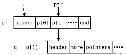
Let’s assume we have gone through the first array p[0] in p and now want to begin traversing p[1], which we rename q. In order to move on to p[2] after we finish with q we will need some stored information—a stack-based algorithm might push p and the current index 1 onto the stack. A variable-size stack is needed rather than some constant amount of memory because this information has to be stored at every level of the arbitrarily-deep traversal. We don’t want to use such a stack, but there is a redundant value we can use: the pointer p[1]=q stored in p. When we finish traversing q and come back to p, we know the address of q, since we just traversed it! So we can safely overwrite that address. But all of the other nearby pointers are in use. It would be very difficult to find space for another word. So instead of storing the location of p, we store a slightly different address: ptr, which points to p[1] (we’ll discuss how to recover the pointer p from ptr later). It won’t help to store ptr in p, since it would just point to its own location! Instead we use a temporary variable prev to hold onto it while we traverse q, and store the previous value of prev, which points to a location inside p’s parent, in the location that used to hold q. By the time we begin traversing q’s first child, r, the picture looks like this:
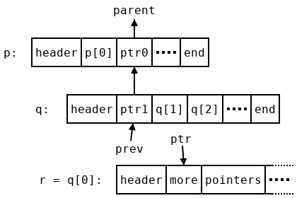
We have reversed all of the pointers above us, and now we have a trail leading all the way back up to the array we started at. To do this we needed an extra temporary value, prev. This uses more memory, but only a constant amount (one word), so it won’t cause problems for us. However, it might be helpful to consider why we need that extra word. In a stack-based traversal only one temporary pointer would be needed to iterate over the array, and in fact we do get away with only writing one word of data in each array during traversal. But the first array doesn’t have any parent array, so there is no pointer to write in it. Instead we write a zero (which is not a valid pointer) to indicate that fact. This zero is an extra word that doesn’t correspond to any array, so to compensate for it we use an extra temporary variable.
When to stop
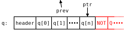
When we finish traversing a pocket, we end up with another problem. We don’t know we’re done! Following the algorithm as described so far, we would end up with ptr pointing at the last element of q, which looks like all of the others, and we would keep moving past the end of q, landing on the header of the next pocket, which probably isn’t even a pointer. Segfault—do not pass go; do not collect the elements of the original array into a list.
A typical algorithm would just store the length of the array on the stack, which we can’t do. However, there is a little more space hiding in the array q which we can use. A pointer gives the location of a particular byte in memory. But the pointers in q all point to the beginning of pockets, which are word-aligned: they begin at addresses which are all multiples of 4 bytes (in 32-bit builds) or 8 bytes (64-bit builds). So we have at least two bits at the bottom of each pointer which are guaranteed to be zero. As long as we remember to clear those bits once we finish, and before following a pointer, we can write anything we want in them!
The first thing to write is a stop bit. We mark the last pointer q with some two bits which aren’t zero (we’ll decide what later). While shuffling pointers around, we always leave the bottom two bits where they were, so that when we get back to q[n] we see the two bits we wrote when we started traversing q. If we haven’t reached the end, that could be anything other than the stop code, and if we have reached the end, it must be the stop code. So now we know when to stop, and won’t segfault by running past the end of a pocket.
However, in order to get back to the parent array with all of our state intact (specifically, the overwritten pointer to the current array), we need to know the address of the beginning of our pocket, not the end. And the shape of the pocket, which we would need to find the pocket’s length, is kept at the beginning of the array as well. How do we get back to the start?
Retracing our steps
Obviously we need to start moving backwards. But once again, we need to know when to stop. Since we’re about to run into it face-first, maybe we should discuss what comes before the pointers in a pocket?

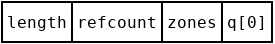
The contents of an array pocket are pretty simple. There are three words at the beginning: the length and reference count of the pocket (which we don’t need to worry about), and the zones field, which contains the type and rank of the pocket along with potentially some other data. Next is the shape (which might be empty!), and then the data in the array—for a nested pocket, pointers to other pockets. There are three cases we want to consider:
- The shape is empty, which means q contains only one pointer. We will run into the zones field right before the last (and first) pointer.
- The shape is not empty, but the total number of pointers is small. We will run into the shape after a short amount of backwards searching.
- The total number of pointers is large. It would take a while to get back to the beginning one pointer at a time, but we also have a lot of spare bits at the bottom of those pointers…
- (Extra credit) The pocket is empty, but it still has a prototype to traverse. For enlist we ignore these pockets, but for other purposes we have to handle this case. The shape has to have a zero in it, but the other axes could have any size that fits in a word.
For the first two cases, we mark the shape and the zones field, respectively. By a lucky coincidence, the bottom two bits of the zones field are used to store the type of the pocket we are in, and for nested arrays, the two bits we care about are always both 1. So let’s make 3 (in binary, 11) the indicator for the zones field. In case 2, the last item of the shape is small, so there are free bits at the top. We’ll shift the shape up to move those to the bottom, leaving room to store the rank and a marker. We’ll choose 1 for the marker.
In case 3, there are enough pointers to store the length of the array in the bottom bits. Since we can’t use the stop marker to encode the length, we opt to just use the bottom bit, that is, storing zeros and ones in the bottom two bits, of each pointer. To distinguish from case 2 we mark the beginning of this offset with a 2, the only unused code so far. We mark the end of the offset with a 2 as well, and then to read the offset we just move backwards, adding each bit to the end of an integer, until we reach that 2. Then we use the length to get back to the beginning of an array. While moving backwards, we also clear those bits to leave the pointers pointing at the exact, byte aligned start of pockets like they did when we found them.
Case 4 is best left as an exercise, I think. There’s a whole empty word in the shape for you to use—what could be easier? Granted, it’s stashed away in some random location in the shape, but that shouldn’t be an obstacle.
Conditions of use
The traversal described above is much faster than trav, but it requires more care to use. Since it scribbles notes on parts of arrays during traversal, the workspace isn’t necessarily in a valid state until it finishes. So it’s not safe to call memory management functions during traversal. Any memory used needs to be allocated before the start of traversal, which means it has to have a constant size: we can’t use anything that will grow as needed.
Enlist is made up of two very simple functions which meet this requirements in most cases: the first goes through and records what types are in the array and how many total elements there are, and the second actually moves the elements into a result array. For the counting function, we just need a little extra storage to fit the type and the count. That’s a constant amount, so it’s fine. For the moving function, we can’t promote an element of a non-mixed array to an element of a mixed array, since this requires us to allocate a new array for it. But this is not a very common case, and when it does happen it will be slow anyway. This means it’s okay to use trav for that case, and use the faster traversal otherwise.
Results
Here are timings showing how long it takes to enlist various arrays, and the improvement from version 15.0 to version 16.0. Timings are measured on a modern CPU, an Intel Kaby Lake i7, but I don’t expect the ratios to change very much on other machines.
| APL expression |
Description |
15.0 |
16.0 |
Ratio |
{(?⍵⍴10){⊂⍵}⌸?⍵⍴99} 1e3 |
1e3 bytes in 10 groups |
6.138E¯7 |
2.898E¯7 |
2.118 |
{(?⍵⍴10){⊂⍵}⌸?⍵⍴99} 1e4 |
1e4 bytes in 10 groups |
1.174E¯6 |
9.439E¯7 |
1.244 |
{(?⍵⍴10){⊂⍵}⌸?⍵⍴99} 1e5 |
1e5 bytes in 10 groups |
8.799E¯6 |
8.168E¯6 |
1.077 |
{⍵⊂⍨1,1↓1=?(≢⍵)⍴2}⍣10?1e4⍴99 |
1e4 bytes nested 10 deep |
8.540E¯4 |
3.464E¯4 |
2.466 |
⊂⍣1e3⊢2 3 |
A 1000-deep nesting |
1.032E¯4 |
1.533E¯5 |
6.730 |
,⍨∘⊂⍣20⊢2 3 |
Duplicated references |
1.648E¯1 |
3.595E¯2 |
4.584 |
The first row is probably the most typical case: a single array with a little bit of nesting, but fairly small leaves. In this case, we can expect to see about a factor of two improvement. As the leaves grow larger, the running time becomes dominated by the time to actually move data to the result, and the improvement falls off, dropping to 25% around 1000 bytes per leaf and 0.8% at 1e4 bytes per leaf. The new code is faster even at very small numbers of leaves. In fact, it takes less time to start up an array traversal than the old method, so it’s many times faster on very deeply nested arrays with few elements in each array. We can see from the final row that the new method has no issues when it encounters the same array many times in one traversal.
The same algorithm is also used for hashing arrays in Dyalog 16.0, which in turn is used for dyadic iota and related functions. The impact on individual operations is not quite as much as the improvements to enlist shown above, but they are still substantial, and being able to search for a few strings in a list more quickly will surely help a lot of applications.


 Follow