
#Dyalog16 – Vibeke Ulmann As announced earlier – and iterated many times by yours truly, to media and other interested parties, because it is SOOOOOOO exciting – this year, the Viking Challenge is to drive a speed boat in the … Continue reading
 Follow
Report from Dyalog ’16 – Monday
Gallery
This gallery contains 9 photos.
This year at the user meeting we have 106 attendees and a further 15 partners and guests, from 15 different countries worldwide. Today was the first day of presentations and the day the user meeting opened formally. Today also saw the arrival of the … Continue reading
Report from Dyalog ’16 – Sunday
Gallery

This gallery contains 10 photos.
It was a gloriously sunny day in Glasgow today. The Golden Jubilee Hotel overlooks the River Clyde and this was the view at sunrise: The day began with delegate registration, with Karen and Fiona manning the registration desk throughout the … Continue reading
Report from Dyalog ’16 – Saturday
Gallery

This gallery contains 4 photos.
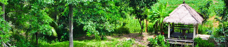
Welcome to Glasgow and to Dyalog ’16 – this year’s annual Dyalog user meeting, which is taking place at the Golden Jubilee Hotel on the banks of the River Clyde. Whether you are attending in Glasgow or following from afar, … Continue reading
APL Exercises
These exercises are designed to introduce APL to a high school senior adept in mathematics. The entire set of APL Exercises has the following sections:
| Introduction 0. Beginnings 1. Utilities 2. Recursion 3. Proofs 4. Rank Operator 5. Index-Of |
6. Key Operator 7. Indexing 8. Grade and Sort 9. Power Operator 10. Arithmetic 11. Combinatorial Objects The Fine Print |
Sections 2 and 10 are the most interesting ones and are as follows. The full set is too lengthy (and too boring?) to be included here. Some students may be able to make up their own exercises from the list of topics. As well, it may be useful to know what the “experts” think are important aspects of APL.
2. Recursion
⎕io←0 throughout.
2.0 Factorial
Write a function to compute the factorial function on integer ⍵, ⍵≥0.
      fac¨ 5 6 7 8
120 720 5040 40320

      n←1+?20
      (fac n) = n×fac n-1
1
      fac 0
1
2.1 Fibonacci Numbers
Write a function to compute the ⍵-th Fibonacci number, ⍵≥0.
      fib¨ 5 6 7 8
5 8 13 21

      n←2+?20
      (fib n) = (fib n-2) + (fib n-1)
1
      fib 0
0
      fib 1
1
If the function written above is multiply recursive, write a version which is singly recursive (only one occurrence of ∇). Use cmpx to compare the performance of the two functions on the argument 35.
2.2 Peano Addition
Let ⍺ and ⍵ be natural numbers (non-negative integers). Write a function padd to compute ⍺+⍵ without using + itself (or - or × or ÷ …). The only functions allowed are comparison to 0 and the functions pre←{⍵-1} and suc←{⍵+1}.
2.3 Peano Multiplication
Let ⍺ and ⍵ be natural numbers (non-negative integers). Write a function ptimes to compute ⍺×⍵ without using × itself (or + or - or ÷ …). The only functions allowed are comparison to 0 and the functions pre←{⍵-1} and suc←{⍵+1} and padd.
2.4 Binomial Coefficients
Write a function to produce the binomal coefficients of order ⍵, ⍵≥0.
      bc 0
1
      bc 1
1 1
      bc 2
1 2 1
      bc 3
1 3 3 1
      bc 4
1 4 6 4 1
2.5 Cantor Set
Write a function to compute the Cantor set of order ⍵, ⍵≥0.
      Cantor 0
1
      Cantor 1
1 0 1
      Cantor 2
1 0 1 0 0 0 1 0 1
      Cantor 3
1 0 1 0 0 0 1 0 1 0 0 0 0 0 0 0 0 0 1 0 1 0 0 0 1 0 1
The classical version of the Cantor set starts with the interval [0,1] and at each stage removes the middle third from each remaining subinterval:
[0,1] →
[0,1/3] ∪ [2/3,1] →
[0,1/9] ∪ [2/9,1/3] ∪ [2/3,7/9] ∪ [8/9,1] → ….

      {(+⌿÷≢)Cantor ⍵}¨ 3 5⍴⍳15
1         0.666667  0.444444   0.296296   0.197531
0.131687  0.0877915 0.0585277  0.0390184  0.0260123
0.0173415 0.011561  0.00770735 0.00513823 0.00342549

      (2÷3)*3 5⍴⍳15
1         0.666667  0.444444   0.296296   0.197531
0.131687  0.0877915 0.0585277  0.0390184  0.0260123
0.0173415 0.011561  0.00770735 0.00513823 0.00342549
2.6 Sierpinski Carpet
Write a function to compute the Sierpinski Carpet of order ⍵, ⍵≥0.
      SC 0
1
      SC 1
1 1 1
1 0 1
1 1 1
      SC 2
1 1 1 1 1 1 1 1 1
1 0 1 1 0 1 1 0 1
1 1 1 1 1 1 1 1 1
1 1 1 0 0 0 1 1 1
1 0 1 0 0 0 1 0 1
1 1 1 0 0 0 1 1 1
1 1 1 1 1 1 1 1 1
1 0 1 1 0 1 1 0 1
1 1 1 1 1 1 1 1 1

      ' ⌹'[SC 3]
⌹⌹⌹⌹⌹⌹⌹⌹⌹⌹⌹⌹⌹⌹⌹⌹⌹⌹⌹⌹⌹⌹⌹⌹⌹⌹⌹
⌹ ⌹⌹ ⌹⌹ ⌹⌹ ⌹⌹ ⌹⌹ ⌹⌹ ⌹⌹ ⌹⌹ ⌹
⌹⌹⌹⌹⌹⌹⌹⌹⌹⌹⌹⌹⌹⌹⌹⌹⌹⌹⌹⌹⌹⌹⌹⌹⌹⌹⌹
⌹⌹⌹   ⌹⌹⌹⌹⌹⌹   ⌹⌹⌹⌹⌹⌹   ⌹⌹⌹
⌹ ⌹   ⌹ ⌹⌹ ⌹   ⌹ ⌹⌹ ⌹   ⌹ ⌹
⌹⌹⌹   ⌹⌹⌹⌹⌹⌹   ⌹⌹⌹⌹⌹⌹   ⌹⌹⌹
⌹⌹⌹⌹⌹⌹⌹⌹⌹⌹⌹⌹⌹⌹⌹⌹⌹⌹⌹⌹⌹⌹⌹⌹⌹⌹⌹
⌹ ⌹⌹ ⌹⌹ ⌹⌹ ⌹⌹ ⌹⌹ ⌹⌹ ⌹⌹ ⌹⌹ ⌹
⌹⌹⌹⌹⌹⌹⌹⌹⌹⌹⌹⌹⌹⌹⌹⌹⌹⌹⌹⌹⌹⌹⌹⌹⌹⌹⌹
⌹⌹⌹⌹⌹⌹⌹⌹⌹         ⌹⌹⌹⌹⌹⌹⌹⌹⌹
⌹ ⌹⌹ ⌹⌹ ⌹         ⌹ ⌹⌹ ⌹⌹ ⌹
⌹⌹⌹⌹⌹⌹⌹⌹⌹         ⌹⌹⌹⌹⌹⌹⌹⌹⌹
⌹⌹⌹   ⌹⌹⌹         ⌹⌹⌹   ⌹⌹⌹
⌹ ⌹   ⌹ ⌹         ⌹ ⌹   ⌹ ⌹
⌹⌹⌹   ⌹⌹⌹         ⌹⌹⌹   ⌹⌹⌹
⌹⌹⌹⌹⌹⌹⌹⌹⌹         ⌹⌹⌹⌹⌹⌹⌹⌹⌹
⌹ ⌹⌹ ⌹⌹ ⌹         ⌹ ⌹⌹ ⌹⌹ ⌹
⌹⌹⌹⌹⌹⌹⌹⌹⌹         ⌹⌹⌹⌹⌹⌹⌹⌹⌹
⌹⌹⌹⌹⌹⌹⌹⌹⌹⌹⌹⌹⌹⌹⌹⌹⌹⌹⌹⌹⌹⌹⌹⌹⌹⌹⌹
⌹ ⌹⌹ ⌹⌹ ⌹⌹ ⌹⌹ ⌹⌹ ⌹⌹ ⌹⌹ ⌹⌹ ⌹
⌹⌹⌹⌹⌹⌹⌹⌹⌹⌹⌹⌹⌹⌹⌹⌹⌹⌹⌹⌹⌹⌹⌹⌹⌹⌹⌹
⌹⌹⌹   ⌹⌹⌹⌹⌹⌹   ⌹⌹⌹⌹⌹⌹   ⌹⌹⌹
⌹ ⌹   ⌹ ⌹⌹ ⌹   ⌹ ⌹⌹ ⌹   ⌹ ⌹
⌹⌹⌹   ⌹⌹⌹⌹⌹⌹   ⌹⌹⌹⌹⌹⌹   ⌹⌹⌹
⌹⌹⌹⌹⌹⌹⌹⌹⌹⌹⌹⌹⌹⌹⌹⌹⌹⌹⌹⌹⌹⌹⌹⌹⌹⌹⌹
⌹ ⌹⌹ ⌹⌹ ⌹⌹ ⌹⌹ ⌹⌹ ⌹⌹ ⌹⌹ ⌹⌹ ⌹
⌹⌹⌹⌹⌹⌹⌹⌹⌹⌹⌹⌹⌹⌹⌹⌹⌹⌹⌹⌹⌹⌹⌹⌹⌹⌹⌹
3-D analogs of the Cantor set and the Sierpinski carpet are the Sierpinski sponge or the Menger sponge.
2.7 Extended H
Write a function for the extend H algorithm for ⍵, ⍵≥0, which embeds the complete binary tree of depth ⍵ on the plane. In ×H ⍵ there are 2*⍵ leaves, instances of the letter o with exactly one neighbor (or no neighbors for 0=⍵). The root is at the center of the matrix.
      xH¨ ⍳5
┌─┬─────┬─────┬─────────────┬─────────────┐
│o│o-o-o│o   o│o-o-o   o-o-o│o   o   o   o│
│ │     │|   |│  |       |  │|   |   |   |│
│ │     │o-o-o│  o---o---o  │o-o-o   o-o-o│
│ │     │|   |│  |       |  │| | |   | | |│
│ │     │o   o│o-o-o   o-o-o│o | o   o | o│
│ │     │     │             │  |       |  │
│ │     │     │             │  o---o---o  │
│ │     │     │             │  |       |  │
│ │     │     │             │o | o   o | o│
│ │     │     │             │| | |   | | |│
│ │     │     │             │o-o-o   o-o-o│
│ │     │     │             │|   |   |   |│
│ │     │     │             │o   o   o   o│
└─┴─────┴─────┴─────────────┴─────────────┘
Write a function that has the same result as xH but checks the result using the assert utility. For example:
assert←{⍺←'assertion failure' ⋄ 0∊⍵:⍺ ⎕SIGNAL 8 ⋄ shy←0}

xH1←{
  h←xH ⍵
  assert 2=⍴⍴h:
  assert h∊'○ -|':
  assert (¯1+2*1+⍵)=+/'o'=,h:
  ...
  h
}
2.8 Tower of Hanoi

(By André Karwath aka Aka (Own work) [CC BY-SA 2.5 (http://creativecommons.org/licenses/by-sa/2.5)], via Wikimedia Commons)
The Tower of Hanoi problem is to move a set of ⍵ different-sized disks from one peg to another, moving one disk at a time, using an intermediate peg if necessary. At all times no larger disk may sit on top of a smaller disk.
Write a function Hanoi ⍵ to solve the problem of moving ⍵ disks from peg 0 to peg 2. Since it’s always the disk which is at the top of a peg which is moved, the solution can be stated as a 2-column matrix with column 0 indicating the source peg and column 1 the destination peg.
      Hanoi¨ ⍳5
┌───┬───┬───┬───┬───┐
│   │0 2│0 1│0 2│0 1│
│   │   │0 2│0 1│0 2│
│   │   │1 2│2 1│1 2│
│   │   │   │0 2│0 1│
│   │   │   │1 0│2 0│
│   │   │   │1 2│2 1│
│   │   │   │0 2│0 1│
│   │   │   │   │0 2│
│   │   │   │   │1 2│
│   │   │   │   │1 0│
│   │   │   │   │2 0│
│   │   │   │   │1 2│
│   │   │   │   │0 1│
│   │   │   │   │0 2│
│   │   │   │   │1 2│
└───┴───┴───┴───┴───┘
Prove that Hanoi ⍵ has ¯1+2*⍵ rows.
10. Arithmetic
⎕io←0 throughout.
10.0 Primality Testing
Write a function prime ⍵ which is 1 or 0 depending on whether non-negative integer ⍵ is a prime number. For example:
      prime 1
0
      prime 2
1
      prime 9
0
      prime¨ 10 10⍴⍳100
0 0 1 1 0 1 0 1 0 0
0 1 0 1 0 0 0 1 0 1
0 0 0 1 0 0 0 0 0 1
0 1 0 0 0 0 0 1 0 0
0 1 0 1 0 0 0 1 0 0
0 0 0 1 0 0 0 0 0 1
0 1 0 0 0 0 0 1 0 0
0 1 0 1 0 0 0 0 0 1
0 0 0 1 0 0 0 0 0 1
0 0 0 0 0 0 0 1 0 0
10.1 Primes Less Than n
Write a function primes ⍵ using the sieve method which produces all the primes less than ⍵. Use cmpx to compare the speed of primes n and (prime¨⍳n)/⍳n. For example:
      primes 7
2 3 5
      primes 50
2 3 5 7 11 13 17 19 23 29 31 37 41 43 47

      (prime¨⍳50)/⍳50
2 3 5 7 11 13 17 19 23 29 31 37 41 43 47
10.2 Factoring
Write a function factor ⍵ which produces the prime factorization of ⍵, such that ⍵ = ×/factor ⍵ and ∧/ prime¨ factor ⍵ is 1. For example:
      factor 144
2 2 2 2 3 3
      ×/ factor 144
144
      ∧/ prime¨ factor 144
1

      factor 1

      factor 2
2
10.3 pco
Read about the pco function in http://dfns.dyalog.com/n_pco.htm and experiment with it.
      )copy dfns pco

      pco ⍳7
2 3 5 7 11 13 17

      1 pco ⍳10
0 0 1 1 0 1 0 1 0 0
G.H. Hardy states in A Mathematician’s Apology (chapter 14, page 23) that the number of primes less than 1e9 is 50847478. Use pco to check whether this is correct.
10.4 GCD
Write a function ⍺ gcd ⍵ to compute the greatest common divisor of non-negative integers ⍺ and ⍵ using the Euclidean algorithm.
Write a function ⍺ egcd ⍵ to compute the GCD of ⍺ and ⍵ as coefficients of ⍺ and ⍵, such that (⍺ gcd ⍵) = (⍺,⍵)+.×⍺ egcd ⍵.
      112 gcd 144
16
      112 egcd 144
4 ¯3
      112 144 +.× 112 egcd 144
16
10.5 Ring Extension
Z[√k] is the ring of integers Z extended with √k where k is not a perfect square. The elements of Z[√k] are ordered pairs (a,b) which can be interpreted as a+b×√k (a+b×k*0.5).
Write a d-operator ⍺(⍺⍺ rplus)⍵ which does addition in Z[√⍺⍺].
      3 4 (5 rplus) ¯2 7
1 11
Write a d-operator ⍺(⍺⍺ rtimes)⍵ which does multiplication in Z[√⍺⍺].
      3 4 (5 rtimes) ¯2 7
134 13
Both of the above can be done using integer operations only.
10.6 Repeated Squaring I
Write a function ⍺ pow ⍵ that computes ⍺*⍵ using repeated squaring. ⍺ is a number and ⍵ a non-negative integer. Hint: the binary representation of an integer n obtains as 2⊥⍣¯1⊢n.
10.7 Repeated Squaring II
Write a d-operator ⍺(⍺⍺ rpow)⍵ that computes ⍺ raised to the power ⍵ using repeated squaring. ⍺ is in Z[√⍺⍺] and ⍵ is a non-negative integer.
⊃ (5 rtimes)/ 13 ⍴ ⊂ 1 1
2134016 954368
1 1 (5 rpow) 13
2134016 954368
1 ¯1 (5 rpow) 13
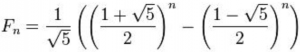
2134016 ¯954368The last two expressions are key steps in an O(⍟n) computation of the n-th Fibonacci number using integer operations, using Binet’s formula:
50847534
⎕io←0 throughout.
I was re-reading A Mathematician’s Apology before recommending it to Suki Tekverk, our summer intern, and came across a statement that the number of primes less than 1e9 is 50847478 (§14, page 23). The function pco from the dfns workspace does computations on primes; ¯1 pco n is the number of primes less than n:
      )copy dfns pco

      ¯1 pco 1e9
50847534
The two numbers 50847478 and 50847534 cannot both be correct. A search of 50847478 on the internet reveals that it is incorrect and that 50847534 is correct. 50847478 is erroneously cited in various textbooks and even has a name, Bertelsen’s number, memorably described by MathWorld as “an erroneous name erroneously given the erroneous value of π(1e9) = 50847478.”
Although several internet sources give 50847534 as the number of primes less than 1e9, they don’t provide a proof. Relying on them would be doing the same thing — arguing from authority — that led other authors astray, even if it is the authority of the mighty internet. Besides, I’d already given Suki, an aspiring mathematician, the standard spiel about the importance of proof.
How do you prove the 50847534 number? One way is to prove correct a program that produces it. Proving pco correct seems daunting — it has 103 lines and two large tables. Therefore, I wrote a function from scratch to compute the number of primes less than ⍵, a function written in a way that facilitates proof.
sieve←{
  b←⍵⍴{∧⌿↑(×/⍵)⍴¨~⍵↑¨1}2 3 5
  b[⍳6⌊⍵]←(6⌊⍵)⍴0 0 1 1 0 1
  49≥⍵:b
  p←3↓{⍵/⍳⍴⍵}∇⌈⍵*0.5
  m←1+⌊(⍵-1+p×p)÷2×p
  b ⊣ p {b[⍺×⍺+2×⍳⍵]←0}¨ m
}

      +/ sieve 1e9
50847534
sieve ⍵ produces a boolean vector b with length ⍵ such that b/⍳⍴b are all the primes less than ⍵. It implements the sieve of Eratosthenes: mark as not-prime multiples of each prime less than ⍵*0.5; this latter list of primes obtains by applying the function recursively to ⌈⍵*0.5. Some obvious optimizations are implemented:
- Multiples of
2 3 5are marked by initializingbwith⍵⍴{∧⌿↑(×/⍵)⍴¨~⍵↑¨1}2 3 5rather than with⍵⍴1. - Subsequently, only odd multiples of primes
> 5are marked. - Multiples of a prime to be marked start at its square.
Further examples:
      +/∘sieve¨ ⍳10
0 0 0 1 2 2 3 3 4 4

      +/∘sieve¨ 10*⍳10
0 4 25 168 1229 9592 78498 664579 5761455 50847534
There are other functions which are much easier to prove correct, for example, sieve1←{2=+⌿0=(⍳3⌈⍵)∘.|⍳⍵}. However, sieve1 requires O(⍵*2) space and sieve1 1e9 cannot produce a result with current technology. (Hmm, a provably correct program that cannot produce the desired result …)
We can test that sieve is consistent with pco and that pco is self-consistent. pco is a model of the p: primitive function in J. Its cases are:
pco n the n-th prime
¯1 pco n the number of primes less than n
1 pco n 1 iff n is prime
2 pco n the prime factors and exponents of n
3 pco n the prime factorization of n
¯4 pco n the next prime < n
4 pco n the next prime > n
10 pco r,s a boolean vector b such that r+b/⍳⍴b are the primes in the half-open interval [r,s).
      ¯1 pco 10*⍳10      ⍝ the number of primes < 1e0 1e1 ... 1e9
0 4 25 168 1229 9592 78498 664579 5761455 50847534

      +/ 10 pco 0 1e9    ⍝ sum of the sieve between 0 and 1e9
50847534
                         ⍝ sum of sums of 10 sieves
                         ⍝ each of size 1e8 from 0 to 1e9
      +/ t← {+/10 pco ⍵+0 1e8}¨ 1e8×⍳10
50847534
                         ⍝ sum of sums of 1000 sieves
                         ⍝ each of size 1e6 from 0 to 1e9
      +/ s← {+/10 pco ⍵+0 1e6}¨ 1e6×⍳1000
50847534

      t ≡ +/ 10 100 ⍴ s
1
                         ⍝ sum of sums of sieves with 1000 randomly
                         ⍝ chosen end-points, from 0 to 1e9
      +/ 2 {+/10 pco ⍺,⍵}/ 0,({⍵[⍋⍵]}1000?1e9),1e9
50847534

      ¯1 pco 1e9         ⍝ the number of primes < 1e9
50847534
      pco 50847534       ⍝ the 50847534-th prime
1000000007
      ¯4 pco 1000000007  ⍝ the next prime < 1000000007
999999937
      4 pco 999999937    ⍝ the next prime > 999999937
1000000007
      4 pco 1e9          ⍝ the next prime > 1e9
1000000007

                         ⍝ are 999999937 1000000007 primes?
      1 pco 999999937 1000000007
1 1
                         ⍝ which of 999999930 ... 1000000009
                         ⍝ are prime?
      1 pco 999999930+4 20⍴⍳80
0 0 0 0 0 0 0 1 0 0 0 0 0 0 0 0 0 0 0 0
0 0 0 0 0 0 0 0 0 0 0 0 0 0 0 0 0 0 0 0
0 0 0 0 0 0 0 0 0 0 0 0 0 0 0 0 0 0 0 0
0 0 0 0 0 0 0 0 0 0 0 0 0 0 0 0 0 1 0 1

      +/∘sieve¨ 999999937 1000000007 ∘.+ ¯1 0 1
50847533 50847533 50847534
50847534 50847534 50847535