Premium Capping Schemes: An important steering Mechanism in German Health Insurance

Blog post from presentation by Dr. Markos Mitsos – Deutsche Krankenversicherung AG DKV – ERGO, Actuarial Department @ Dyalog ’15.

by Vibeke Ulmann

DKV has many million health insurance contracts. Each tariff of each contract has to be checked and possibly adjusted annually in terms of insurance premium based on a number of criteria – without imposing undue ‘financial’ hardship on the Insured individual. Dr. Mitsos is in the process of migrating the simulation modelling into Dyalog APL.

The German Healthcare system is unlike any other in the world. If you earn more than € 45,000 per annum you can choose between the Government Healthcare scheme or draw up a private health insurance. If you are in the state health system you have the option of adding private health insurance on top.

There is legislation in place to ensure that Health insurance companies do not calculate premiums arbitrarily. When entering into a contract the tariff for your health insurance is calculated such that it stays the same over your lifetime. This means that young people pay more than the insurance needs to cover their healthcare expenses whereas older persons are drawing on the reserves that has been saved for them.

The two illustrations below show examples of contract lifetimes

Illustration of correlation between typical annual premiums and claims 07-09-2015

Illustration of  liability high end premium versus annual net premium  and age 07-09-2015

With millions of contracts DSV has Billions of Euro in reserve which they have to manage to the best of their ability. 90% of the proceeds from fund management plus unspent security fees of 5% on each contract has to be paid back to the insurance holders within 3 years and how this is done is the only area where the insurance company has a little freedom to decide how to best distribute the surplus (the socalled “war chest”) to the insurance holders.

If the premium recalculation  shows that some contracts need to have a huge premium increase, DKV, can use part of the  ‘war chest’ to help fund (read cap off) this increase after agreement with an independent Trustee. (Unabhäniger Treuhänder)

The actuary department of DKV – undertakes simulated calculations on the costs of the capping schemes. The results go to the  Executive Board of ERGO and they go to the Chief Actuary in DKV, who is personally liable for the adjustments being in line with the taxation rules, the legislation, and that it is reasonable to impose a premium adjustment accordingly to each individual contract. The final sign off is done by the independent Trustee and then they are implemented into production.

The calculations are typically done on chuncks of around 1 million contracts, and although the maths is ‘simple’ in Actuary terms, the number crunching is massive – thus rendering APL a fast and precise modelling tool for ERGO.

In the ‘old’ days a simulation modelling calculation used to take days. However, according to Dr. Mitsos the simulation calculation done in APL takes mere minutes – and ERGO is  looking into further speeding it up. The actual figures are presented in Excel, and it’s the posting of the number to Excel which actually takes up most of the time.

My main take away from this brilliant presentation –  and subsequent conversation over lunch  – is  the absolutely fantastic number of complex assumptions which have to go into simulating the annual checks and recalculations for premium increases. This becomes especially impressive when you take into consideration that the German Government does NOT allow the Insurance companies to make any forward projections on how they assume/expect a contract will develop in terms of claims over time. Everything has to be calculated ‘as the situation is’ in the year in question.
The way the system is constructed is such that in order to make money as an insurance company you will have to service your customers well.

Parallel Programming with Futures/Isolates

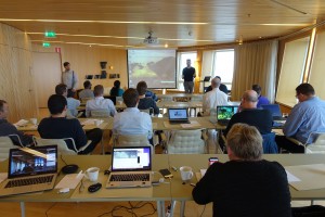
DSC05195Morten Kromberg went right to it with his well-prepared workshop on the prototype features that were introduced in version 14.0 of Dyalog APL. The features are still partly modelled in APL to allow the first wave of users to pass judgement on the design. Throughout the workshop, we were asked for feedback, to ensure that the new primitives will be as well implemented as possible.

Everyone is encouraged to apply the new tools in practice so they can be adjusted and possibly get expanded functionality based on feedback from actual use-cases.

There is no denying the the obvious performance gains that Morten demonstrated: He was able to let the computer waste 9 idle seconds in only slightly more than 3 seconds!

Joking aside, one practical example that showed how useful parallel processing can be, was collating character counts from online news sites. Because of latency in loading these pages over the internet, starting many parallel threads that each requested a page greatly reduced the wait time. DSC05197 One workshop participant volunteered a piece of code that needed to be parallelized got up and pair programmed this with immediately achieving significant performance gains.

The idea of Futures is allowing the continuation of other work before an asynchronously launched calculation is finished. All selection and structural functions can be used on an array containing futures without blocking to wait for the result, as long as no actual data values are required. Meanwhile, other processes (or computers!) could be finishing the evaluation in the background.

It was captivating to observe output being printed and check the status while the calculation work progressed, or accessing parts of an array while other parts still reported as in progress. Morten even had a graphical representation of how load is distributed across processor cores.

Maybe the most exciting thing about all this is that we will soon welcome several new APL squiggles; Isolate (¤) and Parallel (). And at the end of the day, Morten even pulled a pet (pun intended) card out of his sleeve: A Schrödinger’s cat operator! The symbol is of course a question mark in a box (), signifying how the evaluation of the cat’s life (or in our case – the result) does not even begin until actually queried. This is a novel way to specify specific lazy evaluation.

All in all, an exciting look at what possibilities for parallelism the future will bring.

Building a Web Application with MiServer

IMG_4875
One of Sunday’s tracks was Brian Becker’s engaging workshop on MiServer 3.0 – the newest version of Dyalog’s APL-based web application framework that allows you to develop a cross platform application for stand-alone use or delivery via the web.

The motto of MiServer is that everyone who can develop an APL application should also be able to make it available via the web, allowing users to access the application via their favourite browser. In other words, MiServer is browser and platform agnostic.

The main take-away from the morning’s workshop is that if you are used to developing your GUI using ⎕WC, developing the GUI in MiServer 3.0 creates some slightly different rules. First we were showed where to download MiServer, and then Brian guided us though building out very first one-page website. The interactive nature of the workshop captivated us all. Before we knew of it, it was time for lunch.

IMG_4869After lunch – instead of having a sleep inducing talk, Brian challenged us to build a website for a Big Brian’s Burger Bistro offering ordering facility for various products with side orders, and a dashboard to monitor the ordering, product category, speed of order processing, and – most importantly from a management point of view – keep an eye on revenue and which products generate most revenue, with auto update when new orders where processed and paid.

It may have been down to the eating habits of the delegates in terms of their love for burgers, fries etc., but the enthusiasm with which we attacked the challenge was probably more due to how Brian managed to whip up and present MiServer 3.0’s capabilities during the morning. Actually, we got so engrossed in the afternoon that we almost missed our coffee break!

A group of participants was tasked with creating a dashboard, and after some discussion decided on two tables, which would pull data from the business logic, do a bit of calculation, and auto update when new orders got processed.

Hugely entertaining, and we actually managed – courtesy of Rick Proctors swift keyboard handling and deep understanding of APL – to get the code for the dashboard done, working and showcased before we ended the workshop.

We are all looking forward to the MiServer UI Controls presentation on Tuesday morning where we will get a chance to see some the many fancy widgets that MiServer 3.0 offers.


Postcard from Dyalog ’15 – Sicily

IMG_4877We’re here, we’re excited and Naxos greeted us with sweltering temperatures and beautiful sunshine on Saturday. Being the oldest Greek settlement in Sicily, founded before Syracuse, around 735 BC, Naxos has a lot to offer. The Atahotel Naxos venue, where the user meeting is taking place, is situated right on the coast with a fantastic view to the impressive Mount Etna – by far the largest of Europe’s active volcanos.

After some people arriving without luggage, due to huge thunderstorms in Rome both Friday and Saturday, we’re now settled and the luggage issues have been sorted. Today, the weather changed to overcast, thunder and light rain and a more bearable temperature. Which was just as well, as Sunday is WORKSHOP day.

IMG_4894You will find more detailed blog posts from a couple of today’s workshops:

Another noticeable workshop today was Dan Baronet’s Recent Language Features in Practice, covering the recently added operators Rank () and Key ().

Tomorrow the user meeting sessions kick off, and we’re anticipating some hugely interesting and engaging days. This year, the Viking challenge has been swapped for an excursion to Mount Etna, which is scheduled for Wednesday afternoon. Sensible walking shoes recommended. We are looking forward to loads a pictures with ‘thumbs up’ when we get to the top!

Permutations

I started composing a set of APL exercises in response to a query from a new APL enthusiast who attended Morten’s presentation at Functional Conf, Bangalore, October 2014. The first set of exercise are at a low level of difficulty, followed by another set at an intermediate level. One of the intermediate exercises is:

Permutations

a. Compute all the permutations of ⍳⍵ in lexicographic order. For example:

   perm 3
0 1 2
0 2 1
1 0 2
1 2 0
2 0 1
2 1 0

b. Write a function that checks whether is a solution to perm ⍺, without computing perm ⍺. You can use the function assert. For example:

assert←{⍺←'assertion failure' ⋄ 0∊⍵:⍺ ⎕SIGNAL 8 ⋄ shy←0}

pcheck←{
  assert 2=⍴⍴⍵:
  assert (⍴⍵)≡(!⍺),⍺:
  …
  1
}

   6 pcheck perm 6
1

   4 pcheck 2 4⍴0 1 2 3, 0 1 3 2
assertion failure
pcheck[2] assert(⍴⍵)≡(!⍺),⍺:
         ∧

c. What is the index of permutation in perm ⍺? Do this without computing all the permutations. For example:

   7 ip 1 6 5 2 0 3 4    ⍝ index from permutation
1422

(The left argument in this case is redundant, being the same as ≢⍵.)

d. What is the -th permutation of ⍳⍺? Do this without computing all the permutations. For example:

   7 pi 1442             ⍝ permutation from index
1 6 5 2 0 3 4

   (perm 7) ≡ 7 pi⍤0 ⍳!7
1

The Anagram Kata

Coincidentally, Gianfranco Alongi was attempting in APL the anagrams kata from Cyber Dojo:

Write a program to generate all potential anagrams of an input string.

For example, the potential anagrams of “biro” are
biro bior brio broi boir bori
ibro ibor irbo irob iobr iorb
rbio rboi ribo riob roib robi
obir obri oibr oirb orbi orib

This is essentially the same program/exercise/kata, because the potential anagrams are 'biro'[perm 4]. You can compare solutions in other languages to what’s here (google “anagrams kata”).

Spoiler Alert

Deriving a Solution

I am now going to present solutions to part a of the exercise, generating all permutations of ⍳⍵.

Commonly, in TDD (test-driven development) you start with a very simple case and try to extend it successively to more general cases. It’s all too easy to be led into a dead-end because the simple case may have characteristics absent in a more general case. For myself, for this problem, I would start “in the middle”: Suppose I have perm 3, obtained by whatever means:

   p
0 1 2
0 2 1
1 0 2
1 2 0
2 0 1
2 1 0

How do I get perm 4 from that? One way is as follows:

   p1←0,1+p
   (0 1 2 3[p1]) (1 0 2 3[p1]) (2 0 1 3[p1]) (3 0 1 2[p1])
┌───────┬───────┬───────┬───────┐
│0 1 2 3│1 0 2 3│2 0 1 3│3 0 1 2│
│0 1 3 2│1 0 3 2│2 0 3 1│3 0 2 1│
│0 2 1 3│1 2 0 3│2 1 0 3│3 1 0 2│
│0 2 3 1│1 2 3 0│2 1 3 0│3 1 2 0│
│0 3 1 2│1 3 0 2│2 3 0 1│3 2 0 1│
│0 3 2 1│1 3 2 0│2 3 1 0│3 2 1 0│
└───────┴───────┴───────┴───────┘

So it’s indexing each row of a matrix m by 0,1+p. There are various ways of forming the matrix m, one way is:

   ⍒⍤1∘.=⍨0 1 2 3
0 1 2 3
1 0 2 3
2 0 1 3
3 0 1 2

(Some authors waxed enthusiastic about this “magical matrix”.) In any case, a solution obtains readily from the above description: Form a matrix from the above individual planes; replace the 0 1 2 3 by ⍳⍵; and make an appropriate computation for the base case (when 0=⍵). See the 2015-07-12 entry below.

The Best perm Function

What is the “best” perm function I can write in APL? This “best” is a benchmark not only on my own understanding but also on advancements in APL over the years.

“Best” is a subjective and personal measure. Brevity comes into it but is not the only criteria. For example, {(∧/(⍳⍵)∊⍤1⊢t)⌿t←⍉(⍵⍴⍵)⊤⍳⍵*⍵} is the shortest known solution, but requires space and time exponential in the size of the result, and that disqualifies it from being “best”. The similarly inefficient {(∧/(⍳⍵)∊⍤1⊢t)⌿t←↑,⍳⍵⍴⍵} is shorter still, but does not work for 1=⍵.

1981, The N Queens Problem

    p←perm n;i;ind;t
   ⍝ all permutations of ⍳n
    p←(×n,n)⍴⎕io
    →(1≥n)⍴0
    t←perm n-1
    p←(0,n)⍴ind←⍳n
    i←n-~⎕io
   l10:p←(i,((i≠ind)/ind)[t]),[⎕io]p
    →(⎕io≤i←i-1)⍴l10

It was the fashion at the time that functions be written to work in either index-origin and therefore have ⎕io sprinkled hither, thither, and yon.

1987, Some Uses of { and }

   perm:  ⍪⌿k,⍤¯1 (⍙⍵-1){⍤¯ 1 k~⍤1 0 k←⍳⍵
       :  1≥⍵
       :  (1,⍵)⍴0

Written in Dictionary APL, wherein: ⍪⌿⍵ ←→ ⊃⍪⌿⊂⍤¯1⊢⍵ and differs from its definition in Dyalog APL; is equivalent to in dfns; ⍺{⍵ ←→ (⊂⍺)⌷⍵; and ¯ by itself is infinity.

1990-2007

I worked on perm from time to time in this period, but in J rather than in APL. The results are described in a J essay and in a Vector article. The lessons translate directly into Dyalog APL.

2008, http://dfns.dyalog.com/n_pmat.htm

   pmat2←{{,[⍳2]↑(⊂⊂⎕io,1+⍵)⌷¨⍒¨↓∘.=⍨⍳1+1↓⍴⍵}⍣⍵⍉⍪⍬}

In retrospect, the power operator is not the best device to use, because the left operand function needs both the previous result (equivalent to perm ⍵-1) and . It is awkward to supply two arguments to that operand function, and the matter is finessed by computing the latter as 1+1↓⍴⍵.

In this formulation, ⍉⍪⍬ is rather circuitous compared to the equivalent 1 0⍴0. But the latter would have required a or similar device to separate it from the right operand of the power operator.

2015-07-12

   perm←{0=⍵:1 0⍴0 ⋄ ,[⍳2](⊂0,1+∇ ¯1+⍵)⌷⍤1⍒⍤1∘.=⍨⍳⍵}

For a time I thought the base case can be ⍳1 0 instead of 1 0⍴0, and indeed the function works with that as the base case. Unfortunately (⍳1 0)≢1 0⍴0, having a different prototype and datatype.

Future

Where might the improvements come from?

  • We are contemplating an under operator whose monadic case is f⍢g ⍵ ←→ g⍣¯1 f g ⍵. Therefore 1+∇ ¯1+⍵ ←→ ∇⍢(¯1∘+)⍵
  • Moreover, it is possible to define ≤⍵ as ⍵-1 (decrement) and ≥⍵ as ⍵+1 (increment), as in J; whence 1+∇ ¯1+⍵ ←→ ∇⍢≤⍵
  • Monadic = can be defined as in J, =⍵ ←→ (∪⍳⍨⍵)∘.=⍳≢⍵ (self-classify); whence ∘.=⍨⍳⍵ ←→ =⍳⍵

Putting it all together:

   perm←{0=⍵:1 0⍴0 ⋄ ,[⍳2](⊂0,∇⍢≤⍵)⌷⍤1⍒⍤1=⍳⍵}

We should do something about the ,[⍳2] :-)​​

Type Comments

I’ve taken to commenting the closing brace of my inner dfns with a home-grown type notation pinched from the Functional Programming community:

    dref←{                  ⍝ Value for name ⍵ in dictionary ⍺ 
        names values←⍺      ⍝ dictionary pair
        (names⍳⊂⍵)⊃values   ⍝ value corresponding to name ⍵
    }                       ⍝ :: Value ← Dict ∇ Name

I keep changing my mind about whether the result type should be to the left (Value ← ...) or to the right (... → Value). The FP crowd favours → Value but I’m coming around to Value ← because:

* In contrast to (say) Haskell, APL’s function/argument sequences associate right.
* Value ← mirrors the result pattern in a tradfn header and so looks familiar.
* The type of function composition f∘g is simpler this way round.

Such comments serve as an aide-mémoire when I later come to read the code though, with some ingenuity, the notation might possibly be extended to a more formal system, which could have value to a compiler or code-checker. We would need:

Glyphs for Dyalog’s three primitive atomic data types. For no particularly good reason, I’ve been using:

# number
' character
. ref

Glyphs for a few generic (polymorphic) types. These could be just regular lower-case letters a b c … though I currently prefer greek letters:

⍺ ∊ ⍳ ⍴ ⍵ ...

Some constructors for type expressions. This is the most contentious part. For what it’s worth, I’ve been using:

::  is of type ...
∇  function
∇∇  operator
←  returns
[⍺] vector of ⍺s
{⍺} optional left argument ⍺

For example:

foo :: ⍵ ← {⍺} ∇ ⍵

implies:
foo is an ambi-valent function whose
– result is of the same type () as its right argument and whose
– optional left argument may be of a different type ().

I can abstract/name type expressions with (capitalised) identifiers using :=. For example:

Dict   := [Name][Value]        ⍝ dictionary name and value vectors
Eval   := Expr ← Dict ∇ Expr   ⍝ expression reduction
List ⍵ := '∘' | ⍵ (List ⍵)     ⍝ recursive pairs. See
list
Name   := ⍞                    ⍝ primitive type: character vector

The type: character vector ['] is used so frequently that the three glyphs fuse into: . This means that a vector-of-character-vectors, also a common type, is [⍞].

Primitive and derived function types.
If we’re not too nit-picky and ignore issues such as single extension and rank conformability, we can give at least hints for the types of some primitive functions and operators.

 ⍳ :: # ← ⍺ ∇ ⍺              ⍝ dyadic index-of
 ⍴ :: ⍺ ← [#] ∇ ⍺            ⍝ reshape (also take, transpose, ...)

The three forms of primitive composition have interesting types:

∘ :: ⍴ ← {⍺} (⍴ ← {⍺} ∇ ⍳) ∇∇ (⍳ ← ∇ ⍵ ) ⍵     ⍝ {⍺}f∘g ⍵
:: ⍴ ←                 ⍺ ∇∇ (⍴ ← ⍺ ∇ ⍵ ) ⍵   ⍝ A∘g ⍵
:: ⍴ ←      ((⍴ ← ⍺ ∇ ⍵) ∇∇ ⍵ )⍺             ⍝ (f∘B)⍵

It follows that:

f :: ⍴ ← {⍺} ∇ ⍳
g :: ⍳ ←     ∇ ⍵
=> f∘g :: ⍴ ← {⍺} ∇ ⍵          ⍝ intermediate type ⍳ cancels out

and for trains:

A :: ⍳                  ⍝ A is an array of type ⍳
f :: ⍳ ← {⍺} ∇ ⍵
g :: ⍴ ← {⍳} ∇ ∊
h :: ∊ ← {⍺} ∇ ⍵
=> f g h :: ⍴ ← {⍺} ∇ ⍵        ⍝ fgh fork
=> A g h :: ⍴ ←     ∇ ⍵        ⍝ Agh fork
=>   g h :: ⍴ ← {⍺} ∇ ⍵        ⍝ gh atop

For a more substantial example, search function joy for :: and := in a recent download of dfns.dws.

Muse:
This notation is not yet complete or rigorous enough to be of much use to a compiler but there may already be enough to allow the writing of a dfn, which checks its own and others internal consistency. In the long term, if a notation similar to this evolved into something useful, it might be attractive to allow optional type specification as part of the function definition: without the comment symbol:

    dref←{                  ⍝ Value for name ⍵ in dictionary ⍺ 
        names values←⍺      ⍝ dictionary pair
        (names⍳⊂⍵)⊃values   ⍝ value corresponding to name ⍵
    } :: Value ← Dict ∇ Name