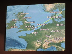
Continuing Morten and Gitte’s whistlestop tour round Europe before heading to the US for DYNA15
From left to right this time…
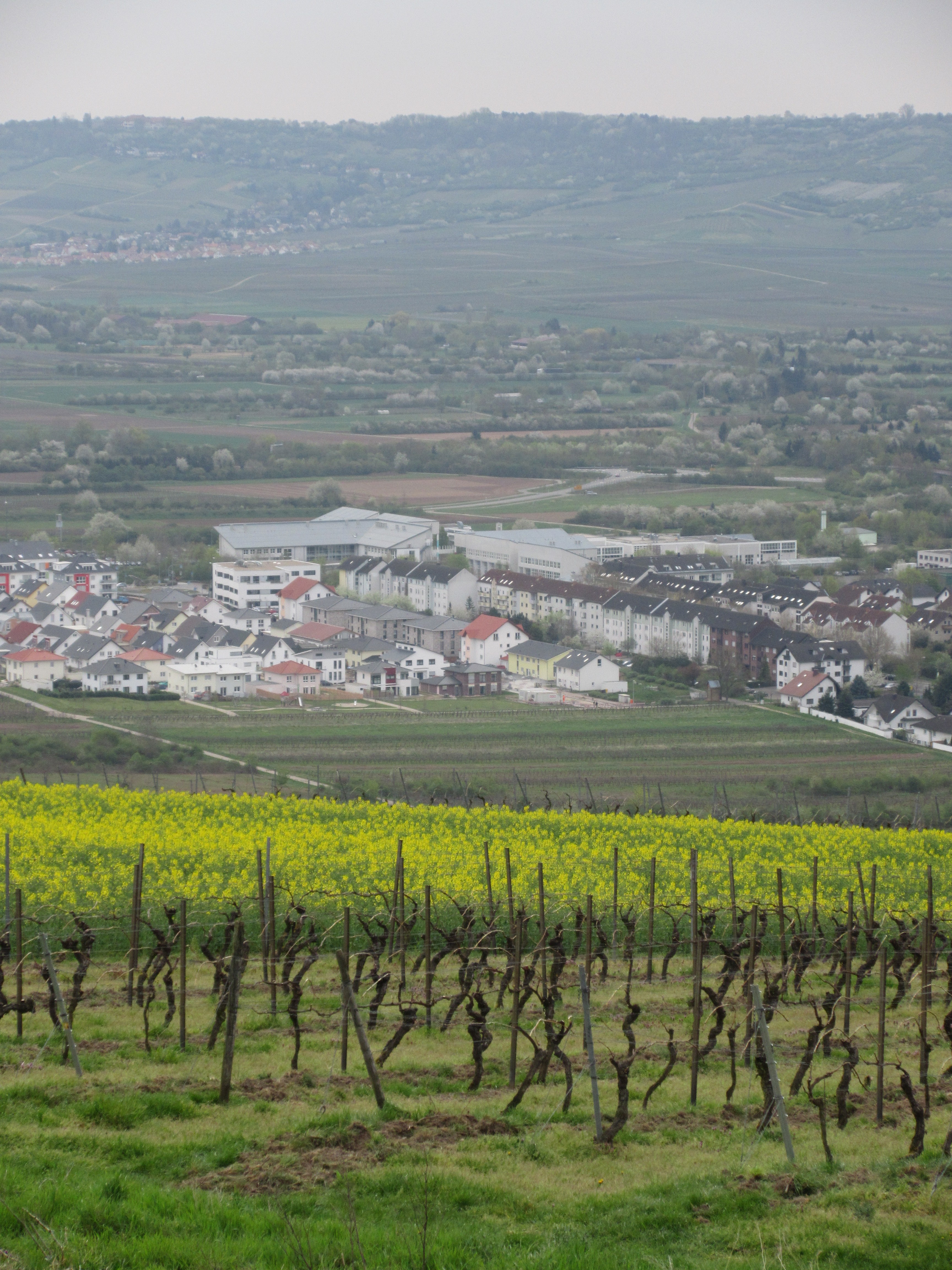
FH Bingen – must have good student parties?
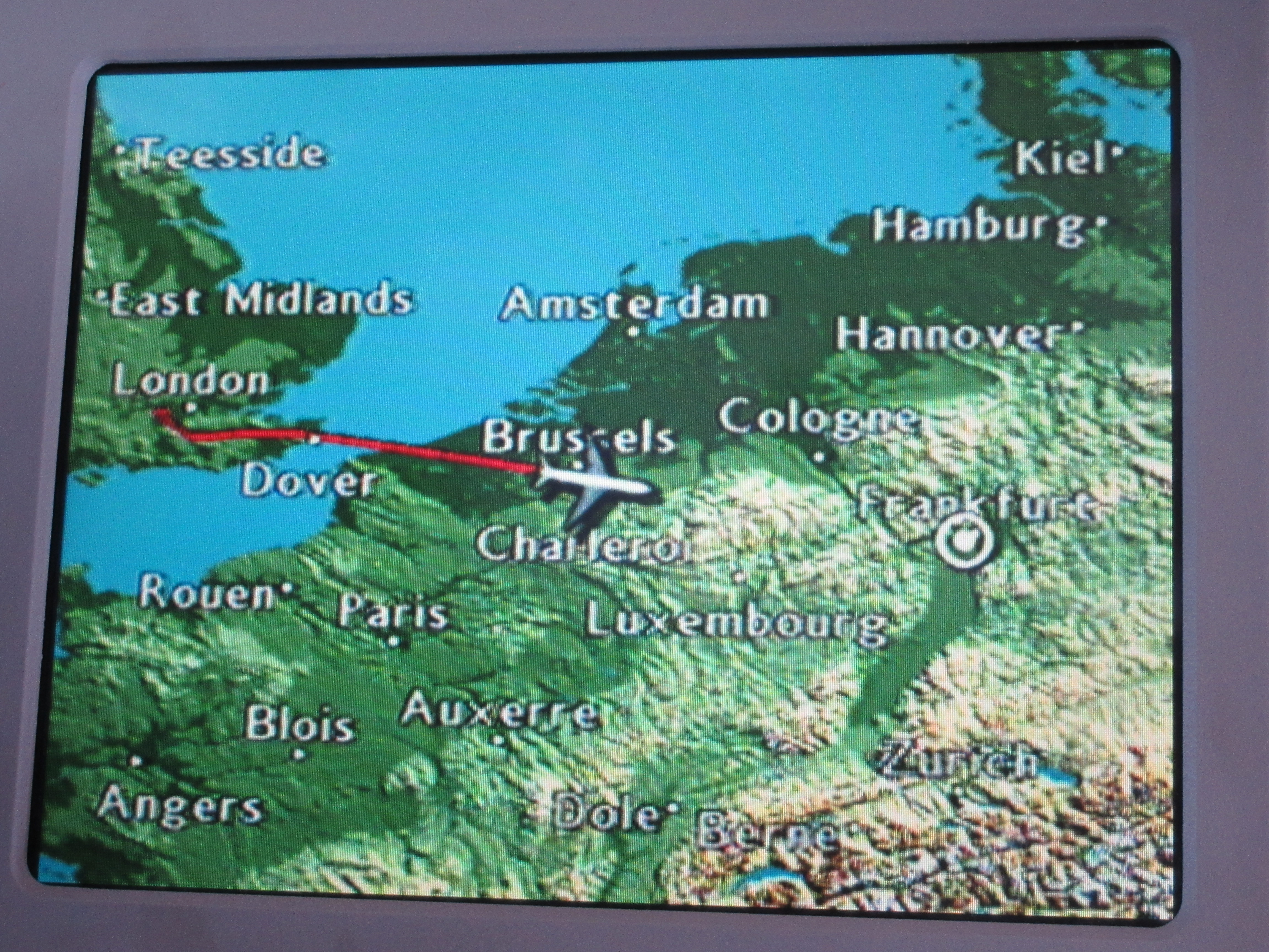
Day 3: Bramley-Bingen
Job interviews done by lunch-time, and we hopped in the car (without lunch) to Heathrow, flew to Frankfurt and finally arrived at Bingen at sunset, just in time for some Weissbier and Flammkücken with the other early arrivals. Bingen is located west of Frankfurt, where the Rhine leaves the plains and bends north through hills, heading for Köln, Düsseldorf and the North Sea. Separated from the river by a vineyard-covered hill lies Fachhochschule Bingen, where our, host Dieter Kilsch, uses APL with MatLab and other tools to teach students about quality control and other subjects.
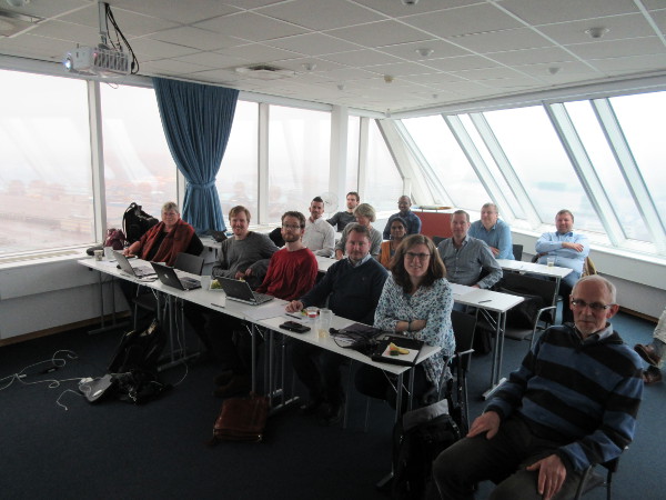
Days 4 & 5: APL Germany Spring Meeting in Bingen
We spent the next two days in the company of about 25 German APL enthusiasts. This time we were first up with a 2.5 hour workshop on Futures and Isolates, and we were very pleased to see that all the delegates who had gone to the trouble of installing Dyalog APL were able to perform all the exercises. We’ll have to make them a little harder next time (Tuesday in Princeton) 🙂 . The afternoon was focused on IBM: News from the Z-series hardware front, and the IBM GSE requirements process, where APL2 users get together and vote on priorities for requests for enhancements. Wouldn’t it be great if our Dyalog users would gang up on us like that and help us to set priorities as a group?
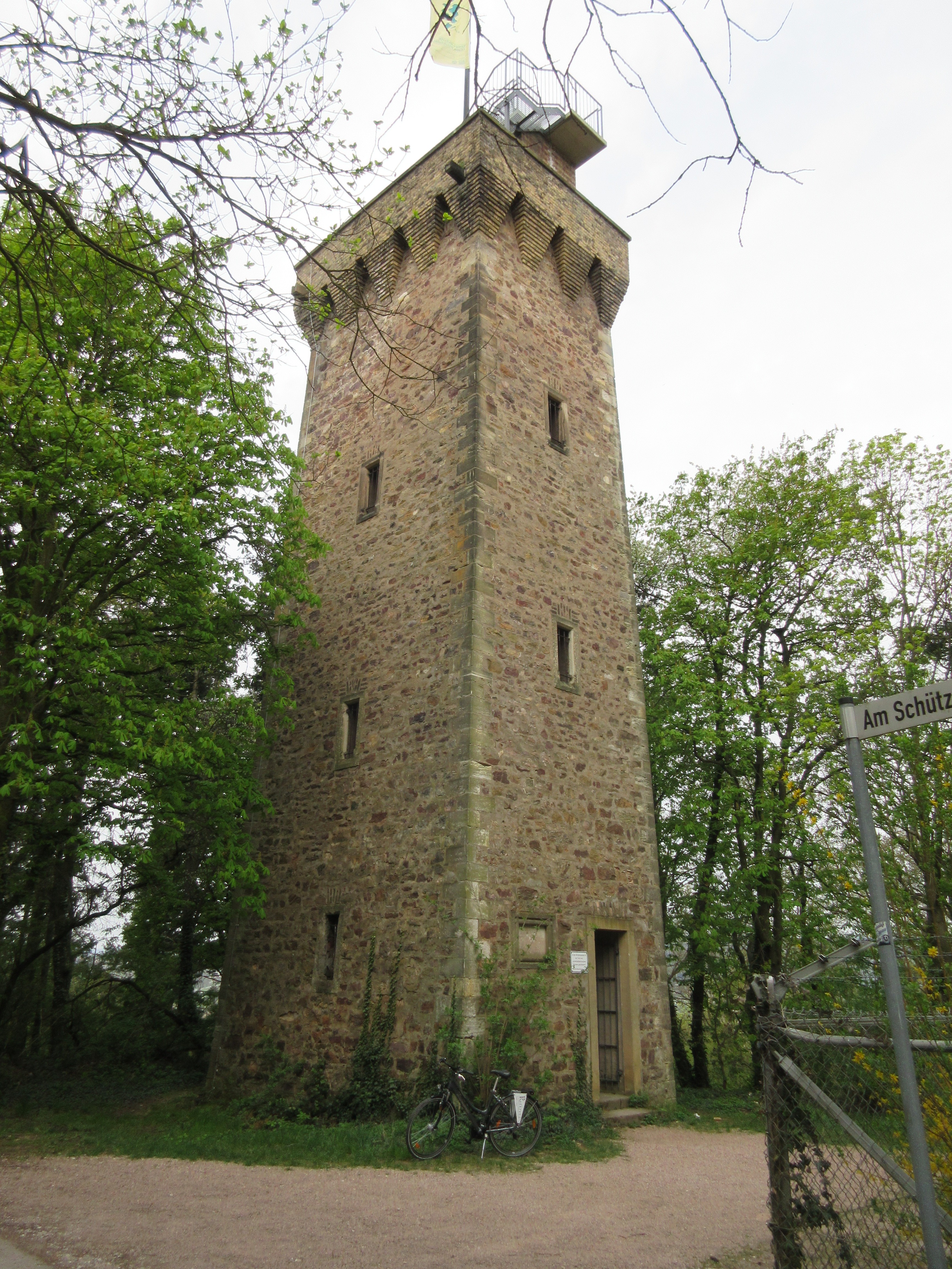
The watch tower at the top of the hill south of Bingen
The first session on Friday was an APL Germany “business session” which we were allowed to skip. Morten discovered that the Tourist Information office next to our hotel rented bikes. They were a little shocked that he was willing to spend €13 for on hour on a bike, but he felt that he really needed to burn some carbon off the spark plugs. Seems he can’t see a hill without feeling it is necessary to make an attempt to get to the top of it.
With Morten energised after an hour on the bike, it was time to return to the meeting. A couple of presentations were particularly interesting: before lunch, Jürgen Sauermann spoke about GNU APL, which is now 2 years old and up to version 1.5. It is very encouraging to see open source APL systems thriving and promoting the use of APL.
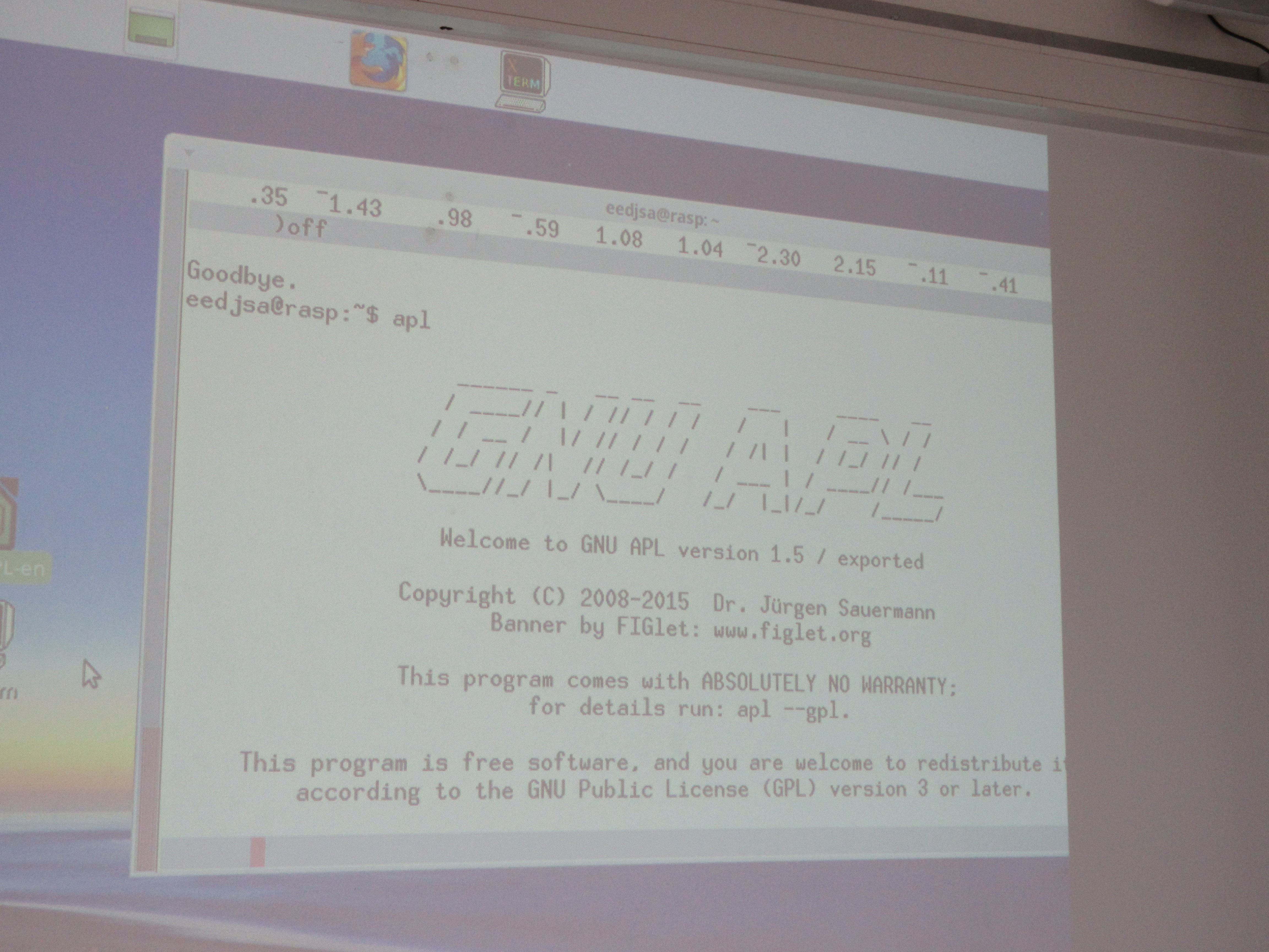
GNU APL
We rounded the two days off with a presentation on our strategy and selected demos of features from versions 14.0 and 14.1: Key, the new experimental JSON parser/generator and the Compiler, threw ourselves in the rental car and headed to Denmark for 15 hours at home before we set off for JFK and Princeton. The story continues next week, on the other side of the Atlantic!
To be concluded…
 Follow