

It seemed like a normal Friday until mid-afternoon. But on 4 February 2022, I embarked on a journey that, at the time, seemed to stretch impossibly far into the future — a future that wasn’t entirely known yet. In the APL Orchard chat room on Stack Exchange, a dozen APLers, some experts and some newbies, held the very first APL Quest chat event.
In this first session, we explored the oldest APL Problem Solving Competition phase 1 problem – question number 1 from 2013 – presented our solutions, and discussed them for about half an hour. The following week, I recorded a video where I went through some of these solutions, with the code posted on GitHub. This pattern continued each week; chat events on Fridays, and a follow-up video released (usually) the week after, each session looking at a different phase 1 problem.
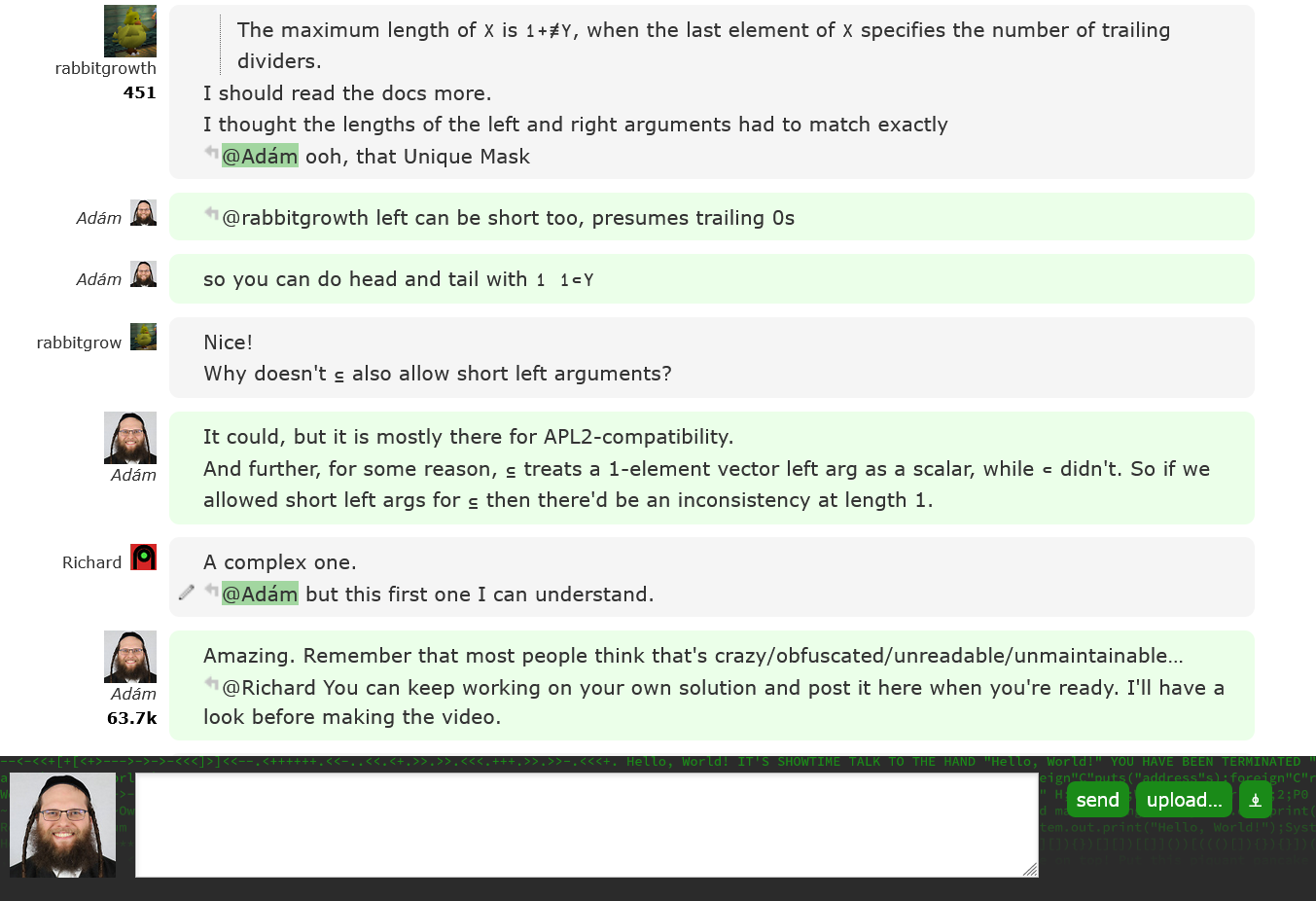
APL Quest chat in progress
Inspiration
Originally, the idea came from Richard Savenije, inspired by LeetCode. Both he and Stefan Kruger, who later became my colleague, were frustrated with LeetCode’s assumptions about programming languages – assumptions that didn’t really hold for APL. Aside from that, their test framework didn’t permit APL submissions anyway.
So, Richard suggested that we should make our own problems website, and Stefan pointed out that my colleague Rich Park had already set up a website that offered automatic checking of solutions to simple problems. With the help of a summer intern, Rich had populated the site with all APL Problem Solving Competition phase 1 problems from 2013 until 2021 (the 2022 round was scheduled to launch two months later). Richard suggested using this site for weekly puzzles, one every Friday afternoon, and we found a time that suited the people present.
Next, we had to decide on a format. Should it be a Zoom meeting or a chat event? Earlier, there had been a couple of chat events series in the APL Orchard; the APL Cultivation series ran weekly from October 2017 until May 2018 and semi-weekly from 28 November 2019 until August 2020. Stefan Kruger was in the process of converting these to a since-completed book, APL Cultivations. After some discussions, we decided to have the sessions in chat, and I came up with the idea of recording a short screen cast after each event.
I got the arithmetic wrong, and claimed we’d have 100 weeks worth of problems, as the 2022 problems would be available by the time we had explored the other problems, giving us almost two years of material. Actually, the 2023 problems were ready when we got to them! But either way, the end seemed very far away…
Technical Details
And yet, here we are, after 110 weeks, 110 live chat events, and 110 published videos – a total of over 22 hours of video contents! We never missed a week, even on various holidays, though Rich Park did have to substitute for me a few times when I was prevented from hosting, and sometimes I had to push off recording and/or publishing a video until two or three weeks after the chat event. Sometimes, I’d host the chat event while travelling in a car or a train, and sometimes I’d record videos in hotel rooms or in other people’s homes. By always using a plain white (or off-white) background, I was able to get a consistent look, irrespective of where I was, though I sometimes had to move furniture to sit in front of a bare wall, and once I had to drape my bedspread over the hotel room’s television…
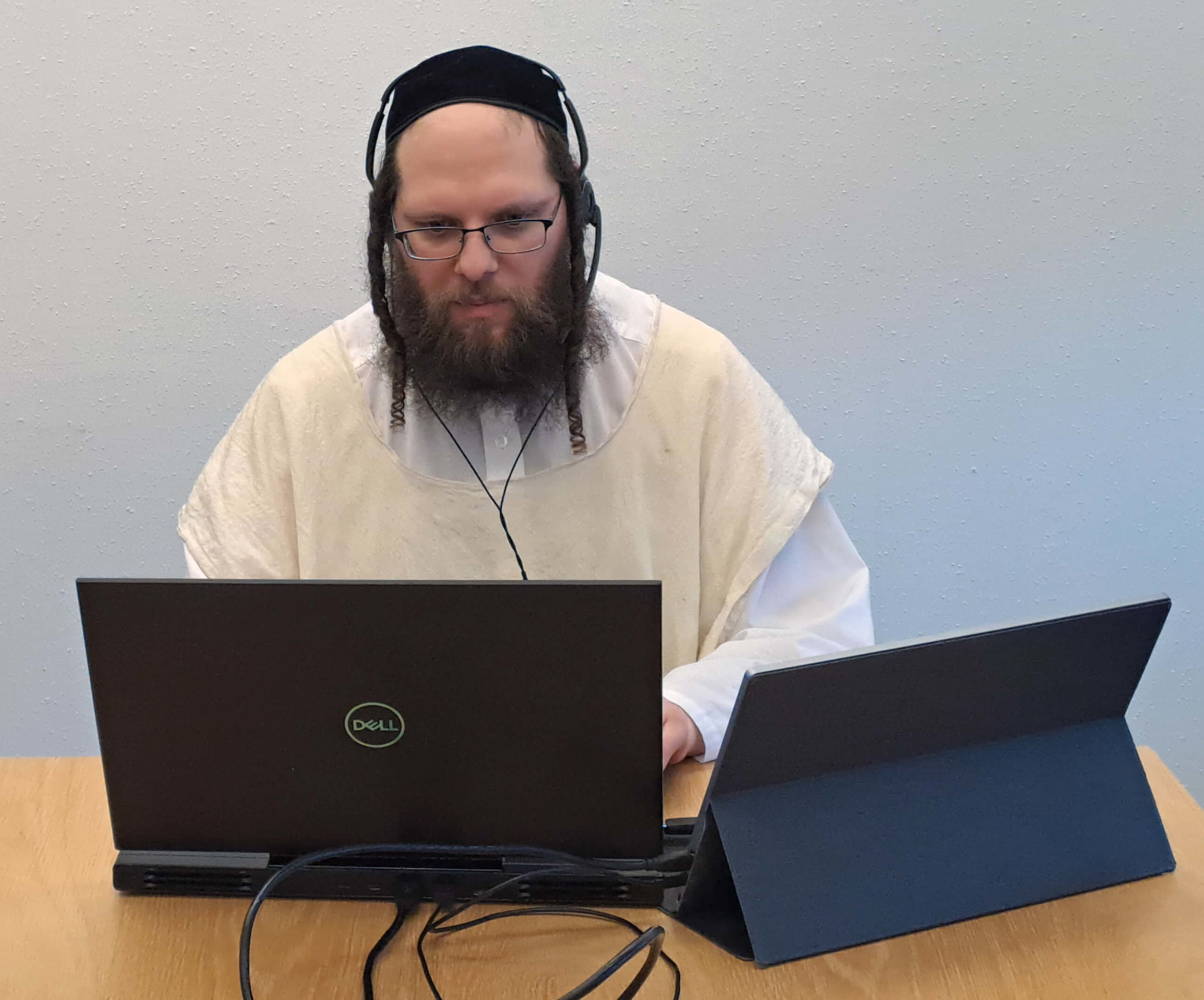
Recording an APL Quest session
Speaking of looks, I’ve received praise for the technical quality of my videos; for their smooth integration of presentation and live coding and for their nice design. So, for those who are interested in how I did it…the introductory screen and the problem statement are simply PowerPoint slides with Fade transitions. After the problem description slide, I faded to a blank slide, and from there, I switched application to RIDE (on Microsoft Windows, you have to install it separately), which was running in full-screen mode with the Language Bar and Status Bar hidden. When I started, the newest released RIDE was version 4.3, but I was running pre-releases of v4.4 and Dyalog v18.2 that added the Nord theme which I had fallen in love with in 2021. By matching my slide colours to the RIDE theme, I achieved a seamless transition without having to do any video editing.
I’m somewhat of a typeface enthusiast. Previously, I had searched for what I considered good sans-serif fonts, and for this project, I choose the humanist Go font. For APL code, I went with my own SAX2 font which I had created by extracting letterforms from the old SAX (SHARP APL for UNIX) manual, and then extended to cover the characters necessary today. However, it bothered me that the SAX font looked so thin next to Go, due to being digitised from the golf ball of a IBM Selectric without accounting for the visual weight normally added by the typewriter’s ink ribbon.
I had to hack font selection into RIDE, which I was able to do because RIDE is built using normal web technology, in particular CSS. After some experimentation, I found the way to do it. After I switched to RIDE v4.5, I was able to set the fontface in an official manner, but even this wasn’t enough. I had relied on PowerPoint’s reasonable auto-bolding of the SAX font, which otherwise didn’t include bold, but RIDE v4.5 wouldn’t let me style the APL font further, so I had to hack RIDE again!
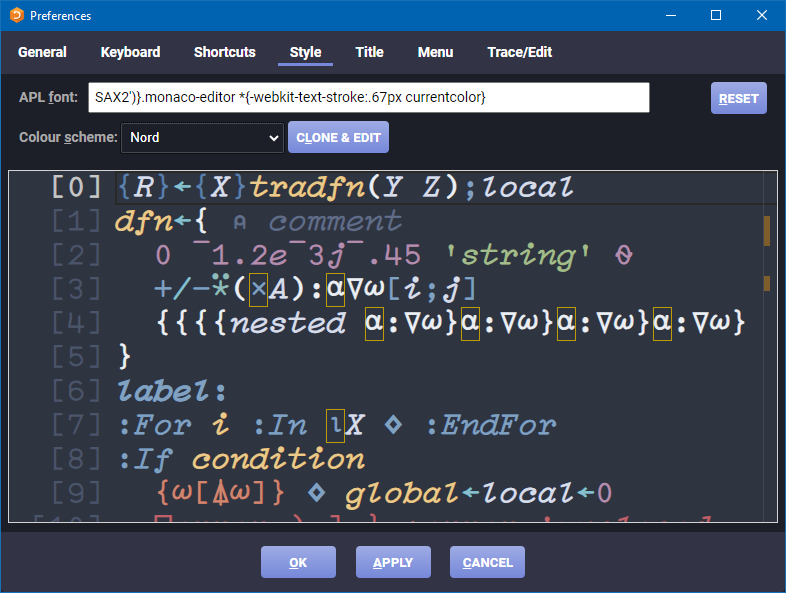
“Hacking” RIDE v4.5
This time, I didn’t need to modify source files, but rather found that RIDE was “vulnerable” (though not in a dangerous way) to CSS injection through its font input field. Making the font bold didn’t look right, as that would only smear the letters horizontally, but adding a “text stroke” had the desired effect. If you want your RIDE to resemble what you can see in the videos, set the APL font to SAX2')}.monaco-editor *{-webkit-text-stroke:.67px currentcolor}. With the visuals set, I recorded using OBS Studio and, on the rare occasion that I needed to edit something, I used DaVinci Resolve.
Concluding the Series
When we finished that last session, it felt rather anti-climactic, but I can look back on a very enjoyable time. And of course, the efforts that all participants put into this are not forgotten; we’ve got an amazing chat and video series that future APLers can enjoy. Thank you to everyone who contributed; chat participants, video commenters, colleagues (especially Brian Becker who authored all the problems), and most of all my wife, who often had to encourage me to record the next video(s) and also gave me the time and space to do so, even if it meant single-handedly keeping our children quiet. If you’re up for a marathon, you can watch the entire 22-hour series on YouTube, and APL Quest on the APL Wiki includes links to all the problems, chat sessions, code, and videos.
 Follow
 After graduating from the University of Portsmouth with a bachelor’s degree in software engineering, Abs started investigating IT roles. He wanted something that provided a challenge, working for a team that was passionate about what they do, and in which he could contribute to that effort through the software and IT abilities that he has accumulated; with Dyalog Ltd he found it! Abs was hurled into the world of APL, which was very different to the Python that he was used to. Although his role doesn’t involve much APL, he appreciates how compact APL solutions can be when wielded correctly. Armed with a fresh perspective and a helpful attitude, he joins our IT department hoping to maintain and improve the current IT infrastructure and provide technical solutions to anyone that needs it.